Excel pivot table replaces staggered display with classic display operation content

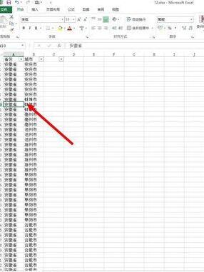
1. Open our data and place the active cell in the data area.

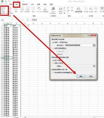
2. Select the inserted pivot table, select the new worksheet display, and click OK.

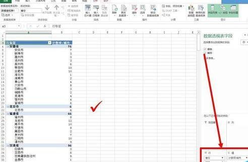
3. Next, we need to drag the data fields to the specified location uniformly to create our pivot table.

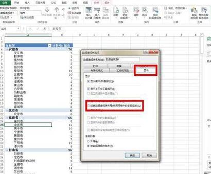
4. Next we need to place the active cell in the data area, right-click and select the PivotTable option.

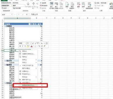
5. After opening, select the display button in the dialog box and select classic display.

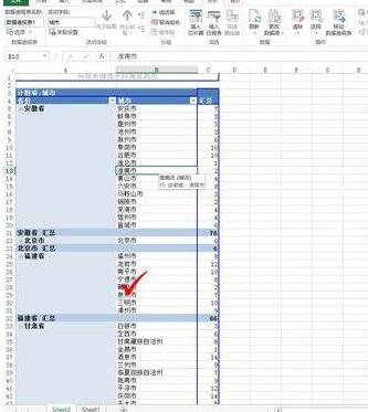
6. After clicking OK, you can see that the display of the pivot table changes to the classic display, and the provinces and cities correspond to each other instead of being scattered.

The above is the detailed content of Excel pivot table replaces staggered display with classic display operation content. For more information, please follow other related articles on the PHP Chinese website!