
 Software TutorialOffice SoftwareCreate a detailed macro with rounded corners in Excel to convert numbers into uppercase
Create a detailed macro with rounded corners in Excel to convert numbers into uppercase

1. How to convert numbers into uppercase and rounded corners in excel?
If you want to convert the numbers in Excel to uppercase with rounded corners, you can do it by following these steps:
1. Prepare data: Enter the numbers that need to be converted in Excel.
2. Open the VBA editor: Press
Alt F11to open the VBA editor.3. Insert a new module: In the VBA editor, right-click any item in the project browser on the left and select "Insert" > "Module ” to insert a new VBA module.
-
4. Write macro code: Write VBA code in a new module, for example:
Function ConvertToWordsWithCents(ByVal MyNumber) Dim Temp Dim DecimalPlace, Count ReDim Place(9) As String Place(2) = " Thousand " Place(3) = " Million " Place(4) = " Billion " Place(5) = " Trillion " ' Convert MyNumber to STRING MyNumber = Trim(CStr(MyNumber)) ' If MyNumber is blank then we're done If MyNumber = "" Then Exit Function ' If MyNumber is 0 then we're done If Val(MyNumber) = 0 Then Exit Function ' Convert MyNumber to hopper DecimalPlace = InStr(MyNumber, ".") If DecimalPlace > 0 Then Temp = GetTens(Left(Mid(MyNumber, DecimalPlace + 1) & "00", 2)) MyNumber = Trim(Left(MyNumber, DecimalPlace - 1)) End If Count = 1 Do While MyNumber <> "" Temp = GetHundreds(Right(MyNumber, 3)) If Temp <> "" Then OutF = Temp & Place(Count) & OutF If Len(MyNumber) > 3 Then MyNumber = Left(MyNumber, Len(MyNumber) - 3) Else MyNumber = "" End If Count = Count + 1 Loop Select Case DecimalPlace Case 0 ConvNumToWordsWithCents = " Dollar " & OutF & "Only" Case 1 ConvNumToWordsWithCents = " Dollar " & OutF & "and " & GetTens(Left(Mid(MyNumber & "00", 2), 2)) & " Cents Only" Case 2 ConvNumToWordsWithCents = " Dollar " & OutF & GetTens(Left(Mid(MyNumber & "00", 2), 2)) & " Cents Only" End Select End Function ' Converts a number from 100-999 into text Function GetHundreds(ByVal MyNumber) Dim Result As String If Val(MyNumber) = 0 Then Exit Function MyNumber = Right("000" & MyNumber, 3) ' Convert the hundreds place. If Mid(MyNumber, 1, 1) <> "0" Then Result = GetDigit(Mid(MyNumber, 1, 1)) & " Hundred " End If ' Convert the tens and ones place. If Mid(MyNumber, 2, 1) <> "0" Then Result = Result & GetTens(Mid(MyNumber, 2)) Else Result = Result & GetDigit(Mid(MyNumber, 3)) End If GetHundreds = Result End Function ' Converts a number from 10 to 99 into text. Function GetTens(TensText) Dim Result As String Result = "" ' Null out the temporary function value. If Val(Left(TensText, 1)) = 1 Then ' If value between 10-19... Select Case Val(TensText) Case 10: Result = "Ten" Case 11: Result = "Eleven" Case 12: Result = "Twelve" Case 13: Result = "Thirteen" Case 14: Result = "Fourteen" Case 15: Result = "Fifteen" Case 16: Result = "Sixteen" Case 17: Result = "Seventeen" Case 18: Result = "Eighteen" Case 19: Result = "Nineteen" Case Else End Select Else ' If value between 20-99... Select Case Val(Left(TensText, 1)) Case 2: Result = "Twenty " Case 3: Result = "Thirty " Case 4: Result = "Forty " Case 5: Result = "Fifty " Case 6: Result = "Sixty " Case 7: Result = "Seventy " Case 8: Result = "Eighty " Case 9: Result = "Ninety " Case Else End Select Result = Result & GetDigit _ (Right(TensText, 1)) ' Retrieve ones place. End If GetTens = Result End Function ' Converts a number from 1 to 9 into text. Function GetDigit(Digit) Select Case Val(Digit) Case 1: GetDigit = "One" Case 2: GetDigit = "Two" Case 3: GetDigit = "Three" Case 4: GetDigit = "Four" Case 5: GetDigit = "Five" Case 6: GetDigit = "Six" Case 7: GetDigit = "Seven" Case 8: GetDigit = "Eight" Case 9: GetDigit = "Nine" Case Else: GetDigit = "" End Select End Function - ##5.
Close the VBA editor: Close the VBA editor and return to Excel.
- 6.
Use a custom function: Use a custom function in Excel ConvertToWordsWithCents
, for example:=ConvertToWordsWithCents(A1)
2. Teach you how to make Excel macros?
You can make Excel macros by following the following steps:- 1.
Open Excel: Open the workbook that contains the macro you want to create.
- 2.
Open the VBA editor: Press Alt F11
to open the VBA editor. - 3.
Insert a new module: In the VBA editor, right-click any item in the project browser on the left and select "Insert" > "Module ” to insert a new VBA module.
- 4.
Write macro code: Write VBA code in a new module. This can include operations on cells, data processing, chart generation, etc.
Sub MyMacro() ' Your VBA code here Range("A1").Value = "Hello, World!" End Sub - 5.
Save Macro: In the VBA editor, click "File" > "Save As", select the file type as "Excel Macro Enabled Work Book (*.xlsm)" and save it.
- 6.
Run macro: In Excel, press Alt F8
to open the macro dialog box, select your macro and click "Run" ".
Summary:
For converting numbers to uppercase with rounded corners, you can write a custom function using VBA, and Called in Excel. The steps to create an Excel macro include opening the VBA editor, inserting a new module, writing macro code, saving the macro, and running the macro. This enables custom functionality and automation.

The above is the detailed content of Create a detailed macro with rounded corners in Excel to convert numbers into uppercase. For more information, please follow other related articles on the PHP Chinese website!

 Microsoft 365 Will Turn Off ActiveX, Because Hackers Keep Using ItApr 12, 2025 am 06:01 AM
Microsoft 365 is finally phasing out ActiveX, a long-standing security vulnerability in its Office suite. This follows a similar move in Office 2024. Beginning this month, Windows versions of Word, Excel, PowerPoint, and Visio in Microsoft 365 will
 How to Use Excel's AGGREGATE Function to Refine CalculationsApr 12, 2025 am 12:54 AM
Quick Links The AGGREGATE Syntax

 How to Format a Spilled Array in ExcelApr 10, 2025 pm 12:01 PM
Use formula conditional formatting to handle overflow arrays in Excel Direct formatting of overflow arrays in Excel can cause problems, especially when the data shape or size changes. Formula-based conditional formatting rules allow automatic formatting to be adjusted when data parameters change. Adding a dollar sign ($) before a column reference applies a rule to all rows in the data. In Excel, you can apply direct formatting to the values or background of a cell to make the spreadsheet easier to read. However, when an Excel formula returns a set of values (called overflow arrays), applying direct formatting will cause problems if the size or shape of the data changes. Suppose you have this spreadsheet with overflow results from the PIVOTBY formula,
 You Need to Know What the Hash Sign Does in Excel FormulasApr 08, 2025 am 12:55 AM
Excel Overflow Range Operator (#) enables formulas to be automatically adjusted to accommodate changes in overflow range size. This feature is only available for Microsoft 365 Excel for Windows or Mac. Common functions such as UNIQUE, COUNTIF, and SORTBY can be used in conjunction with overflow range operators to generate dynamic sortable lists. The pound sign (#) in the Excel formula is also called the overflow range operator, which instructs the program to consider all results in the overflow range. Therefore, even if the overflow range increases or decreases, the formula containing # will automatically reflect this change. How to list and sort unique values in Microsoft Excel
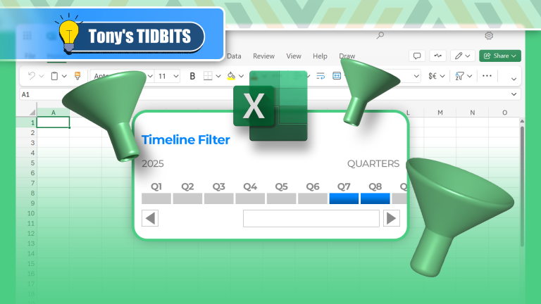 How to Create a Timeline Filter in ExcelApr 03, 2025 am 03:51 AM
In Excel, using the timeline filter can display data by time period more efficiently, which is more convenient than using the filter button. The Timeline is a dynamic filtering option that allows you to quickly display data for a single date, month, quarter, or year. Step 1: Convert data to pivot table First, convert the original Excel data into a pivot table. Select any cell in the data table (formatted or not) and click PivotTable on the Insert tab of the ribbon. Related: How to Create Pivot Tables in Microsoft Excel Don't be intimidated by the pivot table! We will teach you basic skills that you can master in minutes. Related Articles In the dialog box, make sure the entire data range is selected (
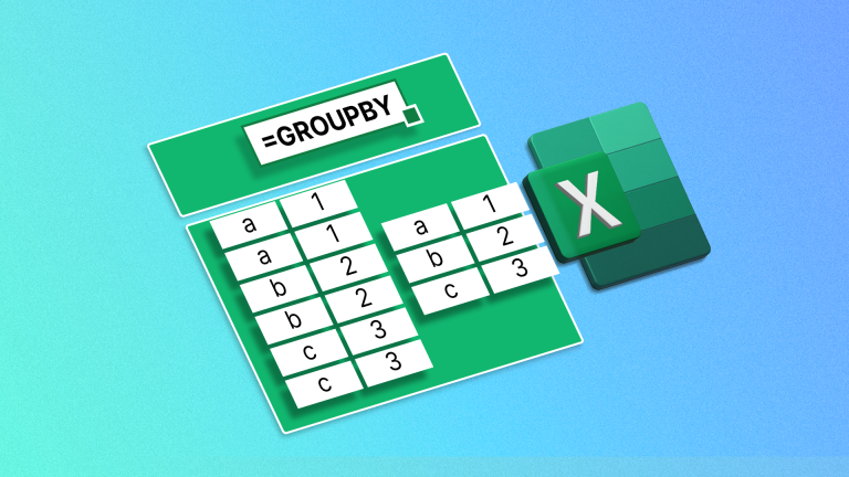 How to Use the GROUPBY Function in ExcelApr 02, 2025 am 03:51 AM
Excel's GROUPBY function: Powerful data grouping and aggregation tools Excel's GROUPBY function allows you to group and aggregate data based on specific fields in a data table. It also provides parameters that allow you to sort and filter the data so that you can customize the output to your specific needs. GROUPBY function syntax The GROUPBY function contains eight parameters: =GROUPBY(a,b,c,d,e,f,g,h) Parameters a to c are required: a (row field): A range (one column or multiple columns) containing the value or category to which the data is grouped. b (value): The range of values containing aggregated data (one column or multiple columns).
 Don't Hide and Unhide Columns in Excel—Use Groups InsteadApr 01, 2025 am 12:38 AM
Excel efficient grouping: say goodbye to hidden columns and embrace flexible data management! While hidden columns can temporarily remove unnecessary data, grouping columns are often a better choice when dealing with large data sets or pursuing flexibility. This article will explain in detail the advantages and operation methods of Excel column grouping to help you improve data management efficiency. Why is grouping better than hiding? Hiding columns (right-click on the column title and select "Hide") can easily lead to data forgetting, even the column title prompt is not reliable because the title itself can be deleted. In contrast, grouped columns are faster and more convenient to expand and fold, which not only improves work efficiency, but also enhances user experience, especially when multi-person collaboration. Additionally, grouping columns allow creation of subgroups, which cannot be achieved by hidden columns. This is the number


Hot AI Tools

Undresser.AI Undress
AI-powered app for creating realistic nude photos

AI Clothes Remover
Online AI tool for removing clothes from photos.

Undress AI Tool
Undress images for free

Clothoff.io
AI clothes remover

AI Hentai Generator
Generate AI Hentai for free.

Hot Article
Hot Tools

Atom editor mac version download
The most popular open source editor

ZendStudio 13.5.1 Mac
Powerful PHP integrated development environment

SublimeText3 Chinese version
Chinese version, very easy to use

WebStorm Mac version
Useful JavaScript development tools

VSCode Windows 64-bit Download
A free and powerful IDE editor launched by Microsoft

