


Excel's GROUPBY function: powerful data grouping and aggregation tools
Excel's GROUPBY function allows you to group and aggregate data based on specific fields in the data table. It also provides parameters that allow you to sort and filter the data so that you can customize the output to your specific needs.
GROUPBY function syntax
The GROUPBY function contains eight parameters:
<code>=GROUPBY(a,b,c,d,e,f,g,h)</code>
Parameters a to c are required:
- a (row field): A range (one column or multiple columns) containing the value or category to which the data is grouped.
- b (value): The range of values containing aggregated data (one column or multiple columns).
- c (function): a function used to aggregate the values in parameter b .
Parameters d to h are optional, and you can learn more about these parameters in the last part of this article:
- d (field title): A number that specifies whether you selected the title in parameters a and b , and whether they should be displayed in the output.
- e (Total Depth): A number that determines whether the output should display the total.
- f (sorting order): a number that indicates how the results are sorted.
- g (Filter Array): An array-oriented formula used to filter out unnecessary information.
- h (field relationship): A number that specifies the field relationship when multiple columns are provided in parameter a .
GROUPBY function practical: only the required parameters are used
If you are overwhelmed by a large number of parameters of the GROUPBY function, it is important to note that GROUPBY function works perfectly even if you only fill in the parameters a , b and c . So first, I'll show you how GROUPBY function can use only these three parameters.
Suppose you have a restaurant chain that serves different dishes from different cuisines and you have calculated the total sales and average customer ratings for each cuisine-dish combination.

While these data are useful, you may be more interested in comparisons of different categories of data. Specifically, you might want to know the total revenue per cuisine and the average customer rating for each dish.
Then, since you want to see the total sales for each cuisine, select the cell that contains these data and add another comma:
<code>=GROUPBY(TabFood[Cuisine],TabFood[Sales],</code>
The last required parameter is the function used for aggregated data. In this example, since you want to find out the total sales of each cuisine, you need to insert the SUM function and turn off the brackets:
<code>=GROUPBY(TabFood[Cuisine],TabFood[Sales],SUM)</code>
After pressing Enter, Excel calculates the average customer rating for each dish type. Again, without any optional parameters, the data is sorted alphabetically by default by the values in the column on the left, with a convenient total row at the bottom.

Since the values in column J are decimal averages, you can organize the displayed decimal places by clicking the "Increase Decimal places" and "Decrease Decimal places" buttons in the "Numbers" group on the Start tab.

GROUPBY function practical: use optional parameters
Although the GROUPBY function has five optional parameters in addition to the three required parameters, which makes it more complicated, these additional options are really just to help you create output that is more in line with your needs. More importantly, you can choose which optional parameters to use and skip unwanted parameters.
Below, I'll cover each optional parameter so you can see how they will affect your data when selecting to include them.
Field title
In my above example, I manually typed the output column headers because by default they are not included in the result. However, if you want the output data to contain the column title and the data it contains, use the field title parameter.
First type your GROUPBY formula, including the first three (required) parameters. In this case, let's assume that you want to group the cuisines by average customer rating:
<code>=GROUPBY(A1:A21,D1:D21,AVERAGE</code>

Note that the title line is included in the selection. In fact, when selecting data for the first two parameters, you should consider in advance whether you want to output the data copy title in the table.
| Benefits of including field titles | Disadvantages of including field titles |
|---|---|
| If you change the title in the original table, the output title will take these changes. | If you want to make the output title more specific than the original table title, you can't change the output title. |
Total depth
The Total Depth parameter allows you to decide whether you want the results to display a total, and if so, whether they should be at the top or bottom of the data. This parameter also allows you to choose whether to display a subtotal.
For Total Depth Parameters, type:
- 0, if you do not want any totals or subtotals to be displayed,
- 1. If you just want to display the total at the bottom of the result,
- 2. If you want the subtotal to appear at the bottom of each result category and display the total at the bottom of the entire result,
- -1, if you just want to display the total at the top of the result,
- -2, if you want the subtotal to appear at the top of each result category and display the total at the top of the entire result.
Sort order
The Sort Order field allows you to tell Excel whether and how to sort the results. Using this parameter does highlight why the GROUPBY function is more useful than using a pivot table: as long as you change any data in the original table, the entire output data is reordered according to the sort order parameters, and the pivot table needs to be refreshed manually.
The number you enter for this parameter represents the column in the result. For example, if you type 1, this will sort the results for the first column in ascending or alphabetical order. On the other hand, typing -1 will sort the results of the first column in descending or inverse alphabetical order.
In this example, I've typed:
<code>=GROUPBY(A1:A21,C1:C21,SUM,,,,-2)</code>
This will sort the second column (sales) in descending order.

Filter arrays
Filtering array parameters are unlikely to be used like the previous optional parameters, although it can help if your original data table contains rows that may break the data.
In this example, the years in cells A2, A8, and A17 interrupt the result of GROUPBY function.

I can use the filter array parameter to tell Excel to ignore any cell containing numbers in column A via the ISNUMBER function:
<code>=GROUPBY(A1:A24,C1:C24,SUM,,,,ISNUMBER(A1:A24)=FALSE)</code>


Field Relationship
Finally, the field relation parameter controls how the data is grouped when the row field parameter refers to multiple columns.
In this example, when the field relationship parameter contains 0 (the default value if the parameter is omitted), GROUPBY will return a hierarchical result table, where each column is represented by a separate data row.
<code>=GROUPBY(A1:B21,C1:C21,SUM,,,3,,0)</code>

On the other hand, when the field relationship parameter contains 1, GROUPBY will return a result table that ignores the hierarchy and sorts each column independently. In other words, categories are not nested, which is why you can't include subtotals in the result when you select this field relationship option.
<code>=GROUPBY(A1:B21,C1:C21,SUM,,,3,,1)</code>

In addition to using SUM and AVERAGE in the GROUPBY function parameters, you can also use the PERENTOF function, which converts data into percentages to show the proportion of the subset that makes up the entire dataset.
The above is the detailed content of How to Use the GROUPBY Function in Excel. For more information, please follow other related articles on the PHP Chinese website!

 Consolidate in Excel: Merge multiple sheets into oneApr 29, 2025 am 10:04 AM
This tutorial explores various methods for combining Excel sheets, catering to different needs: consolidating data, merging sheets via data copying, or merging spreadsheets based on key columns. Many Excel users face the challenge of merging multipl
 Calculate moving average in Excel: formulas and chartsApr 29, 2025 am 09:47 AM
This tutorial shows you how to quickly calculate simple moving averages in Excel, using functions to determine moving averages over the last N days, weeks, months, or years, and how to add a moving average trendline to your charts. Previous articles
 How to calculate average in Excel: formula examplesApr 29, 2025 am 09:38 AM
This tutorial demonstrates various methods for calculating averages in Excel, including formula-based and formula-free approaches, with options for rounding results. Microsoft Excel offers several functions for averaging numerical data, and this gui
 How to calculate weighted average in Excel (SUM and SUMPRODUCT formulas)Apr 29, 2025 am 09:32 AM
This tutorial shows you two simple ways to calculate weighted averages in Excel: using the SUM or SUMPRODUCT function. Previous articles covered basic Excel averaging functions. But what if some values are more important than others, impacting the f
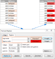 Using Excel Find and Replace in the most efficient wayApr 29, 2025 am 09:07 AM
This tutorial demonstrates how to efficiently locate and modify data within Excel spreadsheets using the Find and Replace function. We'll cover basic and advanced techniques, including wildcard searches and modifications across multiple workbooks. W
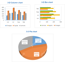 How to make a chart (graph) in Excel and save it as templateApr 28, 2025 am 09:31 AM
This Excel charting tutorial provides a comprehensive guide to creating and customizing graphs within Microsoft Excel. Learn to visualize data effectively, from basic chart creation to advanced techniques. Everyone uses Excel charts to visualize dat
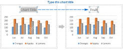 Excel charts: add title, customize chart axis, legend and data labelsApr 28, 2025 am 09:18 AM
After you have created a chart in Excel, what's the first thing you usually want to do with it? Make the graph look exactly the way you've pictured it in your mind! In modern versions of Excel, customizing charts is easy and fun. Microsof
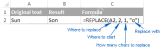 Using Excel REPLACE and SUBSTITUTE functions - formula examplesApr 28, 2025 am 09:16 AM
This tutorial demonstrates the Excel REPLACE and SUBSTITUTE functions with practical examples. Learn how to use REPLACE with text, numbers, and dates, and how to nest multiple REPLACE or SUBSTITUTE functions within a single formula. Last week, we ex


Hot AI Tools

Undresser.AI Undress
AI-powered app for creating realistic nude photos

AI Clothes Remover
Online AI tool for removing clothes from photos.

Undress AI Tool
Undress images for free

Clothoff.io
AI clothes remover

Video Face Swap
Swap faces in any video effortlessly with our completely free AI face swap tool!

Hot Article
Hot Tools

Atom editor mac version download
The most popular open source editor

VSCode Windows 64-bit Download
A free and powerful IDE editor launched by Microsoft

Zend Studio 13.0.1
Powerful PHP integrated development environment

SublimeText3 English version
Recommended: Win version, supports code prompts!

Notepad++7.3.1
Easy-to-use and free code editor

