


Quick Links
- The PIVOTBY Syntax
- PIVOTBY: Using the Required Arguments Only
- PIVOTBY: Using the Optional Arguments
Excel's PIVOTBY function allows you to group your figures without needing to recreate your data in a PivotTable. What's more, data summaries created via PIVOTBY automatically update to reflect changes in your original data, and you can customize what they show by tweaking the formula.
The PIVOTBY SyntaxThe PIVOTBY function lets you input a total of 11 arguments. Although this sounds daunting, the benefit of having so many arguments is that you can tailor the result to align with what you want the data to show.
However, only the first four fields are required.
Required Fields
The required PIVOTBY fields are where you tell Excel which variables you want to be displayed in rows, which variables you want to be displayed in columns, where to find the values, and how you want to aggregate your data:
=PIVOTBY(<em>a</em>,<em>b</em>,<em>c</em>,<em>d</em>)
where
- a are the cells containing the category or categories you want to appear as row headers down the left-hand side of your result,
- b are the cells containing the category or categories you want to appear as column headers across the top of your result,
- c are the values that will appear in the center of your result, according to the rows and columns you selected for arguments a and b, and
- d is the Excel function (or function you've created yourself through LAMBDA) that defines how the data will be aggregated.
The optional PIVOTBY fields allow you to include headers and totals, sort your data, and—in very specific circumstances—specify some additional parameters:
=PIVOTBY(<em>a</em>,<em>b</em>,<em>c</em>,<em>d</em>,[<em>e</em>,<em>f</em>,<em>g</em>,<em>h</em>,<em>i</em>,<em>j</em>,<em>k</em>])
| Argument | What It Is | Notes |
|---|---|---|
| e | A number that specifies whether arguments a, b, and c include headers and whether you want headers to be displayed in the result | 0 = No headers (default) 1 = Headers, but don't show 2 = No headers, but generate them 3 = Headers, and show |
| f | A number that determines whether argument a should contain grand totals and subtotals | 0 = No totals 1 = Grand totals at the bottom (default) 2 = Grand totals and subtotals at the bottom -1 = Grand totals at the top -2 = Grand totals and subtotals at the top |
| g | A number indicating how the columns should be sorted | The number refers to the columns in argument a, followed by the column in argument c. For example, if you had two columns in argument a, "2" would sort the result by the second column of this argument, and "3" would sort the result by argument c. A positive number represents alphabetical or ascending order, and a negative number represents the reverse. |
| h | A number that determines whether argument b should contain grand totals and subtotals | 0 = No totals 1 = Grand totals on the right (default) 2 = Grand totals and subtotals on the right -1 = Grand totals on the left -2 = Grand totals and subtotals on the left |
| i | A number that indicates how the rows should be sorted | The number refers to the columns in argument b, followed by the column in argument c, and works in the same way as argument g. |
| j | A logical expression or formula that lets you filter out rows containing certain values or text | N/A |
| k | A number that gives you more control over how the result's calculations are performed when you use the PERCENTOF function in argument d | 0 = Column totals (default) 1 = Row totals 2 = Grand total 3 = Parent column total 4 = Parent row total |
PIVOTBY: Using the Required Arguments Only
First, let me show you how to use the PIVOTBY function in its simplest form with just the four required fields.
Let's say you've been handed this table of data named Sports_Viewers. It shows the live viewing figures (column D) for six sports (column B) across four regions (column C) over four years (column A), and you've been asked to generate a summary of total viewers by sport and year.


How to Name a Table in Microsoft Excel
"Table1" doesn't explain much...
You could use the GROUPBY function to do this, though you would need to use optional arguments to produce a result that makes analysis easier. What's more, since GROUPBY only sorts data into rows, you could end up with a long list of information that is difficult to interpret.

Instead, using the PIVOTBY function lets you take one or more of the variables and place them into columns, giving you a clearer picture of how your numbers stack up.
PIVOTBY: Using the Optional ArgumentsWhenever you create an Excel formula, each argument is separated by a comma. This means that if you want to skip over any of the optional arguments, you simply need to type a first comma to open the argument, followed by a second comma to close it. The fact that there's nothing between these two commas tells Excel that you've deliberately omitted this argument, so you want the program to adopt the default setting.

The Beginner’s Guide to Excel’s Formulas and Functions
Everything you need to know about Excel's engine room.
1Example 1: Grand Totals and Subtotals
One way to make the PIVOTBY result in the previous example clearer would be to add subtotal rows for each sport.
To do this, you need to type:
=PIVOTBY(Sports_Viewers[[Sport]:[Region]],Sports_Viewers[Year],Sports_Viewers[Viewers],SUM,,2)
Notice how, after argument d (SUM), two commas indicate that you want to jump over argument e (headers), but include argument f (in this case, 2 means that you want to include a subtotal at the bottom of each sport, as well as grand totals at the bottom of the overall result).

Now, let's look at another way to manipulate your result: sorting by one of the output columns.
Typing:
=PIVOTBY(Sports_Viewers[[Sport]:[Region]],Sports_Viewers[Year],Sports_Viewers[Viewers],SUM,,2,3)
means that, after skipping over argument e, as well as including grand totals and subtotals (number 2 in argument f), you also want to order your data by overall viewing figures in ascending order (number 3 in argument g).

Notice how sorting by total viewing figures places not only the sports in order according to their overall totals, but also the regional subcategories according to their subtotals.
Example 3: Percentages (PERCENTOF)
Here's how to view your result using percentages.
Typing:
=PIVOTBY(Sports_Viewers[Sport],Sports_Viewers[Year],Sports_Viewers[Viewers],PERCENTOF,,,2,,,,2)
tells Excel that you want the sports as the row headers (argument a), the years as the column headers (argument b), and you want to aggregate your data (argument c) in the form of percentages (argument d). The first 2 (argument g) represents the order, which, in this case, is by the values. Finally, the second 2 (argument k) tells Excel that the percentages should be relative to the overall data. The unpopulated commas tell Excel you want it to adopt the default for arguments e, f, h, i, and j.


Use the PERCENTOF Function to Simplify Percentage Calculations in Excel
Handle percentages like a pro!
Now, select the cells containing the decimalized results, and click the "Percent Style" icon in the Number group of the Home tab on the ribbon. While you're there, click the "Increase Decimal" and "Decrease Decimal" buttons to define the number of decimal places.
Select extra rows beneath the result in case more data is added to the original table in the future.

Finally, take a moment to digest what this result tells you.

For example, the number of people watching softball in 2022 constitutes 11.5% of the overall viewing figures for all sports across all years. Also, because the data is organized by the total column in ascending order, you can see that nearly a quarter (23.7%) of the overall viewing figures came from people watching basketball.
As well as using SUM, AVERAGE, and PERCENTOF for the function argument in PIVOTBY, you can also use other aggregation functions, like COUNT, MIN, or MAX.
The above is the detailed content of How to Use the PIVOTBY Function in Excel. For more information, please follow other related articles on the PHP Chinese website!

 I Use Custom Number Formatting Instead of Conditional Formatting in ExcelMay 06, 2025 am 12:56 AM
Detailed explanation of custom number formats: Quickly create personalized number formats in Excel Excel provides a variety of data formatting tools, but sometimes built-in tools are not able to meet specific needs or are inefficient. At this point, custom digital formats can come in handy to quickly create digital formats that meet your needs. What is a custom number format and how it works? In Excel, each cell has its own number format, which you can view by selecting the cell and in the Number group on the Start tab of the ribbon. Related: Excel's 12 digital format options and their impact on data Adjust the number format of the cell to match its data type. You can click on the "Number Format" dialog launcher and then
 How to Use the CHOOSECOLS and CHOOSEROWS Functions in Excel to Extract DataMay 05, 2025 am 03:02 AM
Excel's CHOOSECOLS and CHOOSEROWS functions simplify extracting specific columns or rows from data, eliminating the need for nested formulas. Their dynamic nature ensures they adapt to dataset changes. CHOOSECOLS and CHOOSEROWS Syntax: These functio
 How to Use AI Function in Google SheetsMay 03, 2025 am 06:01 AM
Google Sheets' AI Function: A Powerful New Tool for Data Analysis Google Sheets now boasts a built-in AI function, powered by Gemini, eliminating the need for add-ons to leverage the power of language models directly within your spreadsheets. This f
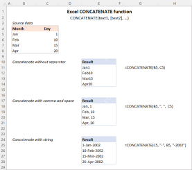 Excel CONCATENATE function to combine strings, cells, columnsApr 30, 2025 am 10:23 AM
This article explores various methods for combining text strings, numbers, and dates in Excel using the CONCATENATE function and the "&" operator. We'll cover formulas for joining individual cells, columns, and ranges, offering solutio
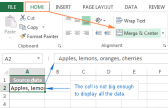 Merge and combine cells in Excel without losing dataApr 30, 2025 am 09:43 AM
This tutorial explores various methods for efficiently merging cells in Excel, focusing on techniques to retain data when combining cells in Excel 365, 2021, 2019, 2016, 2013, 2010, and earlier versions. Often, Excel users need to consolidate two or
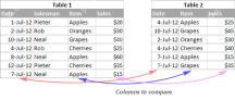 Excel: Compare two columns for matches and differencesApr 30, 2025 am 09:22 AM
This tutorial explores various methods for comparing two or more columns in Excel to identify matches and differences. We'll cover row-by-row comparisons, comparing multiple columns for row matches, finding matches and differences across lists, high
 Rounding in Excel: ROUND, ROUNDUP, ROUNDDOWN, FLOOR, CEILING functionsApr 30, 2025 am 09:18 AM
This tutorial explores Excel's rounding functions: ROUND, ROUNDUP, ROUNDDOWN, FLOOR, CEILING, MROUND, and others. It demonstrates how to round decimal numbers to integers or a specific number of decimal places, extract fractional parts, round to the
 Consolidate in Excel: Merge multiple sheets into oneApr 29, 2025 am 10:04 AM
This tutorial explores various methods for combining Excel sheets, catering to different needs: consolidating data, merging sheets via data copying, or merging spreadsheets based on key columns. Many Excel users face the challenge of merging multipl


Hot AI Tools

Undresser.AI Undress
AI-powered app for creating realistic nude photos

AI Clothes Remover
Online AI tool for removing clothes from photos.

Undress AI Tool
Undress images for free

Clothoff.io
AI clothes remover

Video Face Swap
Swap faces in any video effortlessly with our completely free AI face swap tool!

Hot Article
Hot Tools

Dreamweaver Mac version
Visual web development tools

VSCode Windows 64-bit Download
A free and powerful IDE editor launched by Microsoft

SublimeText3 Chinese version
Chinese version, very easy to use

MinGW - Minimalist GNU for Windows
This project is in the process of being migrated to osdn.net/projects/mingw, you can continue to follow us there. MinGW: A native Windows port of the GNU Compiler Collection (GCC), freely distributable import libraries and header files for building native Windows applications; includes extensions to the MSVC runtime to support C99 functionality. All MinGW software can run on 64-bit Windows platforms.

SecLists
SecLists is the ultimate security tester's companion. It is a collection of various types of lists that are frequently used during security assessments, all in one place. SecLists helps make security testing more efficient and productive by conveniently providing all the lists a security tester might need. List types include usernames, passwords, URLs, fuzzing payloads, sensitive data patterns, web shells, and more. The tester can simply pull this repository onto a new test machine and he will have access to every type of list he needs.

