
 Software TutorialOffice SoftwareI Use Custom Number Formatting Instead of Conditional Formatting in Excel
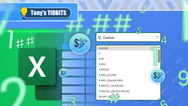
Detailed explanation of custom number formats: Quickly create personalized number formats in Excel
Excel provides a variety of data formatting tools, but sometimes built-in tools are not able to meet specific needs or are inefficient. At this point, custom digital formats can come in handy to quickly create digital formats that meet your needs.
What is a custom number format and how it works?
In Excel, each cell has its own number format, which you can view by selecting the cell and in the Number group on the Start tab of the ribbon.


Related: Excel's 12 digital format options and their impact on data
Adjust the number format of the cell to match its data type.
You can access custom number formats by clicking on the "Number Format" dialog launcher and then clicking "Custom" in the "Set Cell Format" dialog box.

Time is tight? Use these Excel tips to speed up your work
Use Excel's time-saving tools to get the job done.
Before introducing some examples, let's explain how custom number formats work.
Customize the number formats are entered in the Type field in the Custom section of the "Customize" dialog box.

The code you need to insert here follows a strict order:
<code>POSITIVE;NEGATIVE;ZERO;TEXT</code>
In other words, the first parameter in the custom number format field determines the format of the positive number, the second parameter determines the format of the negative number, the third parameter determines the format of the zero, and the fourth parameter determines the format of the text. Also note that semicolons are used to separate each parameter.
For example, enter:
<code>#.00;(#.00);-;"TXT"</code>
Will display:
- Positive numbers are displayed as numbers with two decimal places (#.00).
- Negative numbers are displayed as numbers with two decimal places and enclosed in brackets (#.00).
- Zero is shown as a short horizontal line (-),
- All text values are displayed as the alphabetical string "TXT" ("TXT").

If you omit any parameters by adding a semicolon but not entering any code, the relevant cells in the spreadsheet will appear blank.
For example, enter:
<code>#.00;;;"TXT"</code>
A positive number is displayed as a number with two decimal places, a negative number and a zero are displayed as blank cells, and all text values are displayed as "TXT".

The actual value of the cell remains the same even if the value displayed in each cell depends on what you specify in the Custom Number Format Type field. In the example above, even if cell C2 is displayed as blank (because I omitted the "negative number" parameter in the "Type" field), when I select the cell, the formula bar shows its true value.

This means that I can still use this cell in the formula if I want.

Related: Getting Started with Excel Formulas and Functions
Everything you need to know about Excel engine.
In addition to using custom numeric formats to change the values displayed in the cell, you can also change the color of the values and add symbols to visualize your data. Let's study it in more detail.
Change font color with custom number format
Microsoft Excel's custom number format allows you to define the color of the value in the selected cell. What’s more, for the main eight colors (black, white, red, green, blue, yellow, magenta, and cyan), you don’t need to remember any codes – you can simply type the color name. The color must be the first parameter of each data type and must be placed in square brackets.
Let's look at this example, which shows whether ten employees have met their sales targets. You want all positive numbers in column C to be green, negative numbers to be red and zero to be blue.

To do this, select cell C2, open the Format Cell dialog box (Ctrl 1), and go to the Customize section.
In the Type field, enter:
<code>[Green]#;[Red]#;[Blue]0;</code>
Tell Excel to keep positive and negative numbers as they are (#) — but formatted in green and red, respectively — and format zeros as "0" — but formatted in blue. Since there is no text in this range, you do not need to specify a numeric format for the text value, so only the first three parameters are required.
When you click OK, you will see the text color change accordingly. You can then click and drag the fill handle to the last row of the data to apply this custom number format to the remaining values. This does not change the values in column C, because they are calculated using formulas.

If you want to use a color other than the standard eight colors provided, instead of typing the color name in square brackets, type the color code:

For example, type:
<code>[Color10]#;[Color30]#;[Color16]0;</code>
Use dark green fonts for positive numbers, dark red fonts for negative numbers, and gray fonts for zeros.
Display symbols using custom numeric format
Just like using conditional formatting, you can display symbols based on the corresponding values through custom numeric formats.
Let's use the same example as above, suppose you now want to convert the numbers in the "Result" column (Column C) into an upward arrow for a positive number, a downward arrow for a negative number, and an equal sign (=) for a zero.
To do this, you first need to find the symbols, or know their keyboard shortcuts.
In the Insert tab, click Symbols and insert the symbols in another area of the spreadsheet so that you can copy and paste them into your custom code.

Set font colors, numbers, and symbols with custom number formatting
Now, it is time to combine all the steps mentioned above to produce results showing both colored symbols and arrows.
In the Type field of cell C2, type:
<code>[Green]#▲;[Red]#▼;0" =";</code>
in:
- The first parameter ([Green]#▲) turns the positive value to green, and displays the number and the upward triangle.
- The second parameter ([Red]#▼) turns the negative value into red, and displays the numbers and the downward triangle.
- The third parameter (0" =") has no color format (so in manual cell format) and displays the number "0" followed by a space and the "=" symbol.

To align the number to the left side of the cell and align the symbol to the right side of the cell, type an asterisk (*) and a space between the symbol and the number in each parameter (for example, [Green]#* ▲;[Red]#* ▼;0* " =";). The asterisk tells Excel to repeat the following characters infinitely (until the cell boundary is encountered), and since the following characters are spaces, the gap between the number and symbol changes as the cell width changes.
In the last example, suppose you have calculated the percentage change in the total points for various sports teams, and you want to quickly format positive and negative numbers so that they turn green or red with up or down arrows, including numbers, and are considered percentages. You also want zeros to appear as short horizontal lines.

To do this, in the Type field of the C cell, type:
<code>[Green]▲#%;[Red]▼#%;"-"</code>
Here are the results you will get:

Once you practice adding colors and symbols to cells using custom number formats, you will realize how fast and easy the process is – and, hopefully, you can use custom number formats more often in the future!
The above is the detailed content of I Use Custom Number Formatting Instead of Conditional Formatting in Excel. For more information, please follow other related articles on the PHP Chinese website!

 Time formatting in Excel: 12/24 hour, custom, defaultMay 07, 2025 am 10:42 AM
This tutorial explains the basics and beyond of the Excel time format. Microsoft Excel has a handful of time features and knowing them in depth can save you a lot of time. To leverage powerful time functions, it helps to know how Excel st
 Excel date functions - formula examples of DATE, TODAY, etc.May 07, 2025 am 09:03 AM
This is the final part of our Excel Date Tutorial that offers an overview of all Excel date functions, explains their basic uses and provides lots of formula examples. Microsoft Excel provides a ton of functions to work with dates and ti
 RAND and RANDBETWEEN functions to generate random numbers in ExcelMay 07, 2025 am 09:02 AM
The tutorial explains the specificities of the Excel random number generator algorithm and demonstrates how to use RAND and RANDBETWEEN functions to generate random numbers, dates, passwords and other text strings in Excel. Before we delv
 5 Excel Tips for Power UsersMay 07, 2025 am 12:55 AM
Excel efficiency improvement: Five practical tips to help you process tables quickly Even users who have been using Microsoft Excel for decades can always discover new techniques to improve efficiency. This article shares five practical Excel tips I have accumulated over the years to help you speed up your spreadsheet workflow. 1. No need to freeze the first line: Use Excel tables cleverly When working with Excel tables containing a lot of data, you may get used to freezing the first row through the View tab so that the header is always visible when scrolling. But in fact, if you format the data as an Excel table, you don't need this step. First, make sure that the first row of the data contains the column title. Then, select the data and click "Table" in the "Insert" tab. 2.
 I Use Custom Number Formatting Instead of Conditional Formatting in ExcelMay 06, 2025 am 12:56 AM
Detailed explanation of custom number formats: Quickly create personalized number formats in Excel Excel provides a variety of data formatting tools, but sometimes built-in tools are not able to meet specific needs or are inefficient. At this point, custom digital formats can come in handy to quickly create digital formats that meet your needs. What is a custom number format and how it works? In Excel, each cell has its own number format, which you can view by selecting the cell and in the Number group on the Start tab of the ribbon. Related: Excel's 12 digital format options and their impact on data Adjust the number format of the cell to match its data type. You can click on the "Number Format" dialog launcher and then
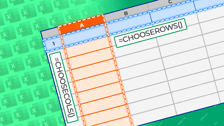 How to Use the CHOOSECOLS and CHOOSEROWS Functions in Excel to Extract DataMay 05, 2025 am 03:02 AM
Excel's CHOOSECOLS and CHOOSEROWS functions simplify extracting specific columns or rows from data, eliminating the need for nested formulas. Their dynamic nature ensures they adapt to dataset changes. CHOOSECOLS and CHOOSEROWS Syntax: These functio
 How to Use AI Function in Google SheetsMay 03, 2025 am 06:01 AM
Google Sheets' AI Function: A Powerful New Tool for Data Analysis Google Sheets now boasts a built-in AI function, powered by Gemini, eliminating the need for add-ons to leverage the power of language models directly within your spreadsheets. This f
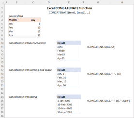 Excel CONCATENATE function to combine strings, cells, columnsApr 30, 2025 am 10:23 AM
This article explores various methods for combining text strings, numbers, and dates in Excel using the CONCATENATE function and the "&" operator. We'll cover formulas for joining individual cells, columns, and ranges, offering solutio


Hot AI Tools

Undresser.AI Undress
AI-powered app for creating realistic nude photos

AI Clothes Remover
Online AI tool for removing clothes from photos.

Undress AI Tool
Undress images for free

Clothoff.io
AI clothes remover

Video Face Swap
Swap faces in any video effortlessly with our completely free AI face swap tool!

Hot Article
Hot Tools

SublimeText3 Chinese version
Chinese version, very easy to use

SublimeText3 Linux new version
SublimeText3 Linux latest version

Dreamweaver Mac version
Visual web development tools

EditPlus Chinese cracked version
Small size, syntax highlighting, does not support code prompt function

MantisBT
Mantis is an easy-to-deploy web-based defect tracking tool designed to aid in product defect tracking. It requires PHP, MySQL and a web server. Check out our demo and hosting services.

