


Quick Links
- The AGGREGATE Syntax
- Example 1: Using AGGREGATE to Ignore Errors
- Example 2: Using AGGREGATE to Ignore Hidden Rows (Reference)
- Example 3: Using AGGREGATE to Ignore Hidden Rows (Array)
- Things to Note When Using the AGGREGATE Function
Excel's AGGREGATE function lets you perform calculations whilst ignoring hidden rows, errors, or other functions that appear in the data. It's similar to the SUBTOTAL function but provides more calculation options and gives you more control over what you want to exclude from the calculation.
The AGGREGATE Syntax
Before we look at some examples of the AGGREGATE function in use, let's see how it works. The AGGREGATE function has two syntaxes—one for references and one for arrays—though you don't need to get yourself tied up in knots over which one you're using, as Excel selects the relevant one depending on the arguments you input. You can see both syntaxes in use when I show you some examples soon.
The Reference Form Syntax
The syntax for the reference form of the AGGREGATE function is:
=AGGREGATE(<em>a</em>,<em>b</em>,<em>c</em>,<em>d</em>)
where
- a (required) is a number that represents the function you want to use in the calculation,
- b (required) is a number that defines what you want the calculation to ignore,
- c (required) is the range of cells on which the function will be applied, and
- d (optional) is the first of up to 252 additional arguments that specify further ranges.
The Array Form Syntax
On the other hand, if you're working with arrays, the syntax is:
=AGGREGATE(<em>a</em>,<em>b</em>,<em>c</em>,<em>d</em>)
where
- a (required) is a number that represents the function you want to use in the calculation,
- b (required) is a number that defines what you want the calculation to ignore,
- c (required) is the array of values on which the function will be applied, and
- d is the second argument required by array functions like LARGE, SMALL, PERCENTILE.INC, and others.
Functions and Exclusions (Arguments a and b)
When entering arguments a and b in either syntax form above, you'll have various options to choose from.
The table below shows the different functions you can use in the AGGREGATE calculation (argument a). Even though you might be tempted to type the function name, remember that this argument must be a number that represents the function you want to use. Functions 1 to 13 are for use with the reference form syntax, and functions 14 to 19 are for use with the array form syntax.
| Number | Function | What It Calculates |
|---|---|---|
| 1 | AVERAGE | The arithmetic mean |
| 2 | COUNT | The number of cells that contain numeric values |
| 3 | COUNTA | The number of cells that are not empty |
| 4 | MAX | The largest value |
| 5 | MIN | The smallest value |
| 6 | PRODUCT | A multiplication |
| 7 | STDEV.S | The simple standard deviation |
| 8 | STDEV.P | The population-based standard deviation |
| 9 | SUM | An addition |
| 10 | VAR.S | The simple variation |
| 11 | VAR.P | The population-based variance |
| 12 | MEDIAN | The middle value |
| 13 | MODE.SNGL | The most frequently occurring number |
| 14 | LARGE | The nth largest value |
| 15 | SMALL | The nth smallest value |
| 16 | PERCENTILE.INC | The nth percentile, with the first and last values included |
| 17 | QUARTILE.INC | The nth quartile, with the first and last values included |
| 18 | PERCENTILE.EXC | The nth percentile, with the first and last values excluded |
| 19 | QUARTILE.EXC | The nth quartile, with the first and last values excluded |
This table lists the numbers you can input to exclude certain values when creating your AGGREGATE formula (argument b):
| Number | What Is Ignored |
|---|---|
| 0 | Nested SUBTOTAL and AGGREGATE functions |
| 1 | Hidden rows, and nested SUBTOTAL and AGGREGATE functions |
| 2 | Errors, and nested SUBTOTAL and AGGREGATE functions |
| 3 | Hidden rows, error values, and nested SUBTOTAL and AGGREGATE functions |
| 4 | Nothing |
| 5 | Hidden rows only |
| 6 | Errors only |
| 7 | Hidden rows and errors |
Now, let's look at some examples of how you can use the AGGREGATE function in real-world scenarios.
Example 1: Using AGGREGATE to Ignore Errors
This Excel spreadsheet contains a list of soccer players, the number of games they've played, the number of goals they've scored, and their game-per-goal ratios. Your aim is to work out the average game-per-goal ratio for all the players combined.

If you were to use the AVERAGE function alone by typing:
=AVERAGE(Player_Goals[Games per goal])
into cell C1, this would return an error, because the referenced range contains #DIV/0! errors.


How to Fix Common Formula Errors in Microsoft Excel
Find out what that error means and how to fix it.
Instead, using the AGGREGATE function gives you the option to ignore these errors and return the average for the remaining data. To do this, in cell C2, you need to type:
=AGGREGATE(1,6,Player_Goals[Games per goal])
where
- 1 (argument a) represents the AVERAGE function,
- 6 (argument b) tells Excel to ignore errors, and
- Player_Goals[Games per goal] is the reference.

Using the same spreadsheet, your next target is to calculate the total number of goals the team has scored.
Example 3: Using AGGREGATE to Ignore Hidden Rows (Array)Next, let's say you wanted to list the two highest goal tallies for players who have played 20 games or fewer.

You could apply the filter first and then generate your formula, but for the purposes of this demonstration, let's create the formula first.
In cell C1, type:
=AGGREGATE(14,5,Player_Goals[Goals scored],{1;2}) where
- 14 (argument a) represents the LARGE function,
- 5 (argument b) tells Excel to ignore hidden rows,
- Player_Goals[Goals scored] is the array of values, and
- {1;2} tells Excel that you want it to return the largest (1) and second-largest values (2) on separate rows (;).
When you press Enter, notice that the result is a spilled array covering cells C1 and C2 because you told Excel to return the top two values.


Everything You Need to Know About Spill in Excel
It's not worth crying over spilled references.
Now, filter the Games Played column to include only those players who have played 20 games or fewer, and see that the result of the AGGREGATE formula you entered earlier changes to ignore the hidden rows.

Things to Note When Using the AGGREGATE Function
Before you go ahead and use the AGGREGATE function in your own Excel workbooks, take a moment to note the following pointers:
- Excel's AGGREGATE function works with vertical ranges only, not horizontal ranges. So, when you reference a horizontal range, AGGREGATE will not ignore rows in hidden columns.
- Argument c in the AGGREGATE formula cannot be the same cell or range of cells across multiple worksheets (also known as 3D references).
- Even though the AGGREGATE function is a great way to bypass errors in calculations, don't get into the habit of ignoring errors altogether. They're there for a reason and could help you troubleshoot issues with your data.
- The array form of the AGGREGATE function will not ignore hidden rows, nested subtotals, or nested aggregates if the array argument includes a calculation.
Another way to hide rows in Excel tables so that the AGGREGATE function only includes what's showing is by inserting slicers, interactive buttons that you can click to make filtering much more straightforward.
The above is the detailed content of How to Use Excel's AGGREGATE Function to Refine Calculations. For more information, please follow other related articles on the PHP Chinese website!

 Time formatting in Excel: 12/24 hour, custom, defaultMay 07, 2025 am 10:42 AM
This tutorial explains the basics and beyond of the Excel time format. Microsoft Excel has a handful of time features and knowing them in depth can save you a lot of time. To leverage powerful time functions, it helps to know how Excel st
 Excel date functions - formula examples of DATE, TODAY, etc.May 07, 2025 am 09:03 AM
This is the final part of our Excel Date Tutorial that offers an overview of all Excel date functions, explains their basic uses and provides lots of formula examples. Microsoft Excel provides a ton of functions to work with dates and ti
 RAND and RANDBETWEEN functions to generate random numbers in ExcelMay 07, 2025 am 09:02 AM
The tutorial explains the specificities of the Excel random number generator algorithm and demonstrates how to use RAND and RANDBETWEEN functions to generate random numbers, dates, passwords and other text strings in Excel. Before we delv
 5 Excel Tips for Power UsersMay 07, 2025 am 12:55 AM
Excel efficiency improvement: Five practical tips to help you process tables quickly Even users who have been using Microsoft Excel for decades can always discover new techniques to improve efficiency. This article shares five practical Excel tips I have accumulated over the years to help you speed up your spreadsheet workflow. 1. No need to freeze the first line: Use Excel tables cleverly When working with Excel tables containing a lot of data, you may get used to freezing the first row through the View tab so that the header is always visible when scrolling. But in fact, if you format the data as an Excel table, you don't need this step. First, make sure that the first row of the data contains the column title. Then, select the data and click "Table" in the "Insert" tab. 2.
 I Use Custom Number Formatting Instead of Conditional Formatting in ExcelMay 06, 2025 am 12:56 AM
Detailed explanation of custom number formats: Quickly create personalized number formats in Excel Excel provides a variety of data formatting tools, but sometimes built-in tools are not able to meet specific needs or are inefficient. At this point, custom digital formats can come in handy to quickly create digital formats that meet your needs. What is a custom number format and how it works? In Excel, each cell has its own number format, which you can view by selecting the cell and in the Number group on the Start tab of the ribbon. Related: Excel's 12 digital format options and their impact on data Adjust the number format of the cell to match its data type. You can click on the "Number Format" dialog launcher and then
 How to Use the CHOOSECOLS and CHOOSEROWS Functions in Excel to Extract DataMay 05, 2025 am 03:02 AM
Excel's CHOOSECOLS and CHOOSEROWS functions simplify extracting specific columns or rows from data, eliminating the need for nested formulas. Their dynamic nature ensures they adapt to dataset changes. CHOOSECOLS and CHOOSEROWS Syntax: These functio
 How to Use AI Function in Google SheetsMay 03, 2025 am 06:01 AM
Google Sheets' AI Function: A Powerful New Tool for Data Analysis Google Sheets now boasts a built-in AI function, powered by Gemini, eliminating the need for add-ons to leverage the power of language models directly within your spreadsheets. This f
 Excel CONCATENATE function to combine strings, cells, columnsApr 30, 2025 am 10:23 AM
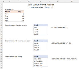
This article explores various methods for combining text strings, numbers, and dates in Excel using the CONCATENATE function and the "&" operator. We'll cover formulas for joining individual cells, columns, and ranges, offering solutio


Hot AI Tools

Undresser.AI Undress
AI-powered app for creating realistic nude photos

AI Clothes Remover
Online AI tool for removing clothes from photos.

Undress AI Tool
Undress images for free

Clothoff.io
AI clothes remover

Video Face Swap
Swap faces in any video effortlessly with our completely free AI face swap tool!

Hot Article
Hot Tools

SublimeText3 Chinese version
Chinese version, very easy to use

SublimeText3 Linux new version
SublimeText3 Linux latest version

Dreamweaver Mac version
Visual web development tools

EditPlus Chinese cracked version
Small size, syntax highlighting, does not support code prompt function

MantisBT
Mantis is an easy-to-deploy web-based defect tracking tool designed to aid in product defect tracking. It requires PHP, MySQL and a web server. Check out our demo and hosting services.

