Tips to Make Excel Sheets Instantly More Attractive

How to make Excel tables more beautiful instantly

1.Change the default table line color

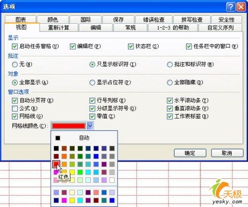
By default, the edges of cells are gray thin dotted lines. However, aesthetic fatigue may occur after long-term use. We can try changing the color of the border lines.

Click the menu command "Tools→Options" to open the "Options" dialog box and select the "View" tab. In the "Gridline Color" drop-down list below, you can reselect the color of the cell border lines, as shown in Figure 1. After confirmation, the color of the grid lines will change.

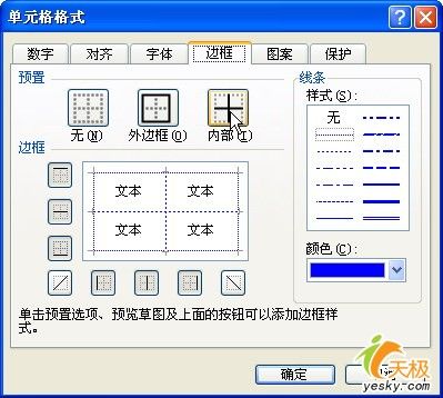
Of course, we can directly select the cell and specify the border line and color for it. The method is to select the cell range and click the menu command "Format → Cells" to open the "Format Cells" dialog box. We can click the "Border" tab, then specify the color and line type of the border line, and specify border lines for the four borders of the cell, as shown in Figure 2. Click the "Pattern" tab to specify a fill color and pattern for the cell.

2. Use automatic format

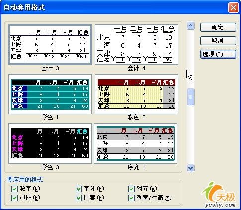
If we don’t want to format the table one by one ourselves, we can select the table area and click the menu command “Format→AutoFormat” to open the “AutoFormat” dialog box. Select a format in the list, as shown in Figure 3. After confirming, you will get the same form immediately. We can also click the "Options" button in the dialog box, and then select among the "Format to be applied" options at the bottom of the dialog box to make the resulting format more suitable for our needs.

How to merge multiple excel tables into one

1. Put multiple excel tables in the same folder, and create a new excel in this folder.

2. Use Microsoft Excel to open the newly created excel sheet, right-click sheet1, find "View Code", and click in. After entering, you will see the macro calculation interface.

3. Then copy the following macro calculation codes, and then find "Run Subprocess/User Form" under "Run" on the toolbar. The code is as follows, as shown in the figure:

Sub merges all worksheets in all workbooks in the current directory ()

Dim MyPath, MyName, AWbName

Dim Wb As Workbook, WbN As String

Dim G As Long

Dim Num As Long

Dim BOX As String

Application.ScreenUpdating = False

MyPath = ActiveWorkbook.Path

MyName = Dir(MyPath & ＂\＂ & ＂*.xls＂)

AWbName = ActiveWorkbook.Name

Num = 0

Do While MyName "＂"

If MyName AWbName Then

Set Wb = Workbooks.Open(MyPath & "\＂" & MyName)

Num = Num 1

With Workbooks(1).ActiveSheet

.Cells(.Range("B65536").End(xlUp).Row 2, 1) = Left(MyName, Len(MyName) - 4)

For G = 1 To Sheets.Count

Wb.Sheets(G).UsedRange.Copy .Cells(.Range(＂B65536＂).End(xlUp).Row 1, 1)

Next

WbN = WbN & Chr(13) & Wb.Name

Wb.Close False

End With

End If

MyName = Dir

Loop

Range(＂B1＂).Select

Application.ScreenUpdating = True

MsgBox "A total of "& Num &" all worksheets under "& Num &" workbooks have been merged. As follows: "& Chr(13) & WbN, vbInformation, "Prompt"

End Sub

4. After running, wait for about 10 seconds. When the running is completed, that is, after the merger is completed, there will be a prompt, just click OK. Looking at the merged data, there are more than 5,000 rows, which is the result of merging data from 17 excel tables in the same folder. The effect is shown in the figure.

How to make excel look more beautiful

Method/Step

1. Edit the table. The table is a student performance table, which contains the scores of four students A, B, C, and D in the three subjects of Chinese, mathematics, and English. You can enter the data and save it.

2. Adjust the font. , use the mouse to frame the table, right-click the mouse, select Format Cells, select the "Font" item, and set it as needed. After setting, select the "Center" option to make the table look neater.

3. Adjust the format. , use the mouse to frame the Chinese, Mathematics and English cells under the subject, right-click the mouse, select Format Cells, select the "Align" item, select "Center Across Columns" for horizontal alignment, and select "Center" for vertical alignment. .

4. Adjust the arrangement. , use the mouse to frame the Chinese, Mathematics and English cells under the subject, right-click the mouse, select Format Cells, select the "Alignment" item, under "Direction", click the text, then the fonts will be sorted vertically. If If you need to tilt it, you can adjust the angle on the right side to set it as needed.

5

5. Add borders. , use the mouse to frame the table, right-click the mouse, select Format Cells, select the "Border" item, and set it as needed.

How to make Excel tables more beautiful

You can also do it according to the following method:

The necessary steps to create an interface table in Excel are to set a unified background color. The gradient is more beautiful than the general single color. The font format must be coordinated with the background color. Add explanatory text under the icon to keep the color of the entire table. Same color family.

Step 1: Fill the entire table with light gray.

The necessary steps to create an interface table in excel are to set a unified background color.

Step 2: Set the white fill color of the row where the icon is placed, then insert the text box to set the gradient color, enter the text and set the font to Chinese color text.

Gradient is more beautiful than ordinary single color, and the font format should be coordinated with the background color.

Step 3: Add icons by copying, pasting or inserting (you can download many beautiful icon materials by searching for "icon" in or image), determine the position of the first and last icon, and then use the picture tool Top-aligned and horizontally-aligned images.

Step 4: Add description text below the icon. Insert text box-input and set font-remove border lines. Finally, use the third step to align the text.

Step 5 (optional): Development Tools - Insert - Frame - Set to three-dimensional format.

Step 6: Add a dark blue scroll above.

The color of the entire table should be kept in the same color system. The scroll above can use gradient colors, and the light color in the middle can make the graphics more three-dimensional.

Step 7: Set up hyperlinks and description text to display when the cursor hovers

Right click-hyperlink-location of this document-select the table, click "Screen Tips" and enter the prompt text.

So far, the interface production is completed

The above is the detailed content of Tips to Make Excel Sheets Instantly More Attractive. For more information, please follow other related articles on the PHP Chinese website!