


Excel's LAMBDA Functions: An easy guide to creating custom functions
Before Excel introduced the LAMBDA function, creating a custom function requires VBA or macro. Now, with LAMBDA, you can easily implement it using the familiar Excel syntax. This guide will guide you step by step how to use the LAMBDA function.
It is recommended that you read the parts of this guide in order, first understand the grammar and simple examples, and then learn practical applications.
The LAMBDA function is available for Microsoft 365 (Windows and Mac), Excel 2024 (Windows and Mac), and Excel for the web. Excel 2019 and earlier does not support this feature.
LAMBDA function syntax
Creating a custom function using LAMBDA requires two parameters:
<code>=LAMBDA(x, y)</code>
in:
-
xis the input variable (up to 253), -
yis the calculation formula.
The input variable ( x ) cannot conflict with cell references, nor can it contain periods; the calculation formula ( y ) is always the last parameter of the LAMBDA function.
Simple example
Enter the following formula in Sheet1 cell A1 in a blank Excel workbook:
<code>=LAMBDA(a,b,a*b)</code>
(Do not press Enter for the time being)

a,b defines variables, and a*b is the calculation formula. If a is 4 and b is 6, the result is 24.
After pressing Enter, a #CALC! error appears because the value has not been assigned yet.


You can test it by adding variable values at the end of the formula:
<code>=LAMBDA(a,b,a*b)(4,6)</code>

After pressing Enter, the cell will display 24.

Although it is easier to enter directly =4*6 , the advantage of LAMBDA is that it can name calculation formulas and reuse them, especially when the calculations are complex. When modifying a formula, you only need to modify the function itself to affect all relevant calculations.
Double-click the cell, select the original LAMBDA formula (the content before the first bracket), and press Ctrl C to copy.

Press the Esc key and click Define Name in the Formula tab.

In the New Name dialog box:
| Fields | illustrate | operate |
|---|---|---|
| name | Name the function | Enter eg SIMPLELAMBDA
|
| Scope | Define the scope of function | Select Workbook |
| illustrate | Function description, displayed as tooltip | Enter a short description |
| Quotation location | Function definition | Delete existing content, press Ctrl V to paste the copied LAMBDA formula |

Click OK. Enter =SIMPLELAMBDA(9,6) in cell A1 and press Enter, and the result is 54.

Cell references can also be used, for example =SIMPLELAMBDA(A1,A2) .

Practical application examples
Suppose you need to create a LAMBDA function that adds 20% VAT in the UK to all costs.

First, enter =B2*1.2 in the first cell.

Double-click the cell and add the LAMBDA function:
<code>=LAMBDA(cost,cost*1.2)(B2)</code>

Copy the LAMBDA formula, click "Define Name", and name it AddVAT .

Delete column C data and enter =AddVAT(B2) in cell C2.

If VAT is reduced to 15%, just modify "1.2" in the function definition to "1.15".

All calculations using the AddVAT function are automatically updated.

Notes when using LAMBDA functions
- The LAMBDA function can only be used in the workbook where it was created.
- The function name must be unique.
- The input variable name cannot conflict with the cell reference, nor can it contain periods, and the number of variables cannot exceed 253.
Excel's LAMBDA function can combine any existing function to perform complex calculations, making it more powerful. Once you master it, you can try more complex calculations.
The above is the detailed content of How to Use LAMBDA in Excel to Create Your Own Functions. For more information, please follow other related articles on the PHP Chinese website!

 I Use Custom Number Formatting Instead of Conditional Formatting in ExcelMay 06, 2025 am 12:56 AM
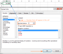
Detailed explanation of custom number formats: Quickly create personalized number formats in Excel Excel provides a variety of data formatting tools, but sometimes built-in tools are not able to meet specific needs or are inefficient. At this point, custom digital formats can come in handy to quickly create digital formats that meet your needs. What is a custom number format and how it works? In Excel, each cell has its own number format, which you can view by selecting the cell and in the Number group on the Start tab of the ribbon. Related: Excel's 12 digital format options and their impact on data Adjust the number format of the cell to match its data type. You can click on the "Number Format" dialog launcher and then
 How to Use the CHOOSECOLS and CHOOSEROWS Functions in Excel to Extract DataMay 05, 2025 am 03:02 AM
Excel's CHOOSECOLS and CHOOSEROWS functions simplify extracting specific columns or rows from data, eliminating the need for nested formulas. Their dynamic nature ensures they adapt to dataset changes. CHOOSECOLS and CHOOSEROWS Syntax: These functio
 How to Use AI Function in Google SheetsMay 03, 2025 am 06:01 AM
Google Sheets' AI Function: A Powerful New Tool for Data Analysis Google Sheets now boasts a built-in AI function, powered by Gemini, eliminating the need for add-ons to leverage the power of language models directly within your spreadsheets. This f
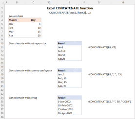 Excel CONCATENATE function to combine strings, cells, columnsApr 30, 2025 am 10:23 AM
This article explores various methods for combining text strings, numbers, and dates in Excel using the CONCATENATE function and the "&" operator. We'll cover formulas for joining individual cells, columns, and ranges, offering solutio
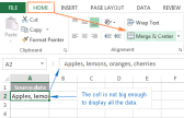 Merge and combine cells in Excel without losing dataApr 30, 2025 am 09:43 AM
This tutorial explores various methods for efficiently merging cells in Excel, focusing on techniques to retain data when combining cells in Excel 365, 2021, 2019, 2016, 2013, 2010, and earlier versions. Often, Excel users need to consolidate two or
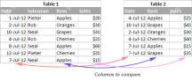 Excel: Compare two columns for matches and differencesApr 30, 2025 am 09:22 AM
This tutorial explores various methods for comparing two or more columns in Excel to identify matches and differences. We'll cover row-by-row comparisons, comparing multiple columns for row matches, finding matches and differences across lists, high
 Rounding in Excel: ROUND, ROUNDUP, ROUNDDOWN, FLOOR, CEILING functionsApr 30, 2025 am 09:18 AM
This tutorial explores Excel's rounding functions: ROUND, ROUNDUP, ROUNDDOWN, FLOOR, CEILING, MROUND, and others. It demonstrates how to round decimal numbers to integers or a specific number of decimal places, extract fractional parts, round to the
 Consolidate in Excel: Merge multiple sheets into oneApr 29, 2025 am 10:04 AM
This tutorial explores various methods for combining Excel sheets, catering to different needs: consolidating data, merging sheets via data copying, or merging spreadsheets based on key columns. Many Excel users face the challenge of merging multipl


Hot AI Tools

Undresser.AI Undress
AI-powered app for creating realistic nude photos

AI Clothes Remover
Online AI tool for removing clothes from photos.

Undress AI Tool
Undress images for free

Clothoff.io
AI clothes remover

Video Face Swap
Swap faces in any video effortlessly with our completely free AI face swap tool!

Hot Article
Hot Tools

Notepad++7.3.1
Easy-to-use and free code editor

Atom editor mac version download
The most popular open source editor

VSCode Windows 64-bit Download
A free and powerful IDE editor launched by Microsoft

WebStorm Mac version
Useful JavaScript development tools

Dreamweaver CS6
Visual web development tools

