
Home >Software Tutorial >Office Software >Excel graphic method for summing based on cell colors
Excel graphic method for summing based on cell colors

- WBOYWBOYWBOYWBOYWBOYWBOYWBOYWBOYWBOYWBOYWBOYWBOYWBforward
- 2024-04-17 18:52:05981browse
Quick method to sum based on cell color Dear readers, have you ever needed to quickly calculate the sum based on the color of Excel cells? PHP editor Banana has brought you a step-by-step graphic tutorial that will guide you to master this clever method easily. This article will introduce in detail how to use Excel's conditional formatting function to filter and sum based on the color of cells to help you manage data efficiently. Come and learn more!
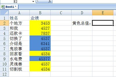
Take the table below as an example to quickly sum the values in the yellow cells.
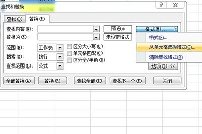
Press CTLR H to bring up the Find and Replace window, click the option next to it, click the small arrow next to the format button of [Find Content], and select [From Unit] in the pop-up menu Select the format].
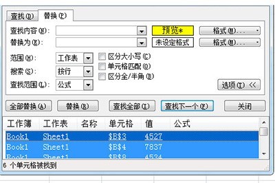
Absorb yellow cells and find them all. Then CTRL A selects all cells in the search box and closes it.
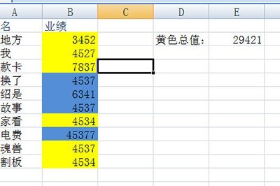
Click [Formula]-[Definition Name] above and enter yellow in it.

Finally, enter the formula =SUM (yellow) in the cell where the sum is required. With a press of Enter, all yellow cell values are summed. Even if the data inside is changed, the summed value will automatically change.
The above is the detailed content of Excel graphic method for summing based on cell colors. For more information, please follow other related articles on the PHP Chinese website!