Detailed method of using formulas to create star charts in Excel

Use formulas to create star charts in Excel? PHP editor Baicao reveals the secret for you! No need for tedious drawing, you can easily create a cool star decoration. Read on to learn the detailed steps!

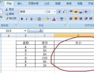
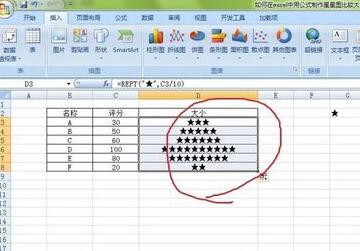
As shown in the picture, I want to use the formula in the size column to create a star chart to compare the size of the rating data in column C.

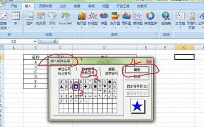
Before operating through the formula, you must first know how to enter the five-pointed star, click Insert, and then select the symbol More

In the pop-up Insert In the Special Symbols dialog box, select Special Symbols, then select the solid five-pointed star and click OK

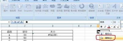
Select the solid five-pointed star and click Copy for later use

Enter the formula =REPT("★",C3/10) in cell D3, and then press Enter

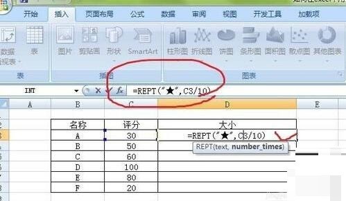
After pressing Enter, the star chart based on the data will appear, and the cell will drop down Copy the formula and the star chart that intuitively reflects the size of the data is completed

The above is the detailed content of Detailed method of using formulas to create star charts in Excel. For more information, please follow other related articles on the PHP Chinese website!