How to use the if multiple function in Excel to create employee annual leave table

php editor Xigua is here to introduce to you how to use the if function in Excel to create an employee annual leave table. The if function is one of the most commonly used functions in Excel. It can judge and filter data based on certain conditions. When making an employee annual leave table, we can use the if function to determine whether the employee's number of leave days meets the annual leave requirements, and fill the results into the corresponding cells. Using the if function can save us time and energy and make making annual leave tables more efficient and accurate. Next, let’s discuss the specific operation methods together!

1. Clarify the relevant regulations and implementation rules for annual leave. That is, employees who have worked for 1 year but less than 10 years in total are entitled to 5 days of annual leave; employees who have been working for 10 years but less than 20 years are entitled to 10 days of annual leave; employees who have been working for 20 years or more are entitled to 15 days of annual leave. Under one of the special circumstances, annual leave cannot be taken.

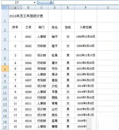
2. Create a new excel form and enter the form name, serial number, job number, name, gender, date of employment and other relevant information.

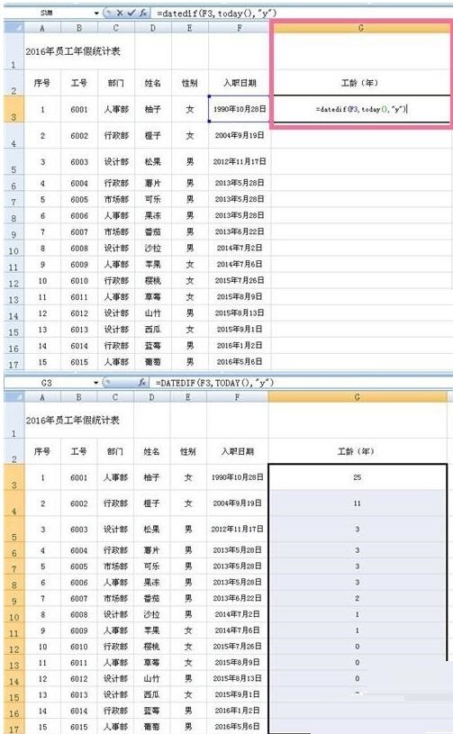
3. Enter [length of service (years)" in cell G2, enter the formula in cell G3: =DATEDIF(F3,TODAY(),"y"), and press [Return] Car/enter] can calculate the employee's length of service. Among them, the DATEDIF function is to calculate the corresponding value from the start date to the end date. In F3, the entry date is the starting time, TODAY() is the current date, and Y is the number of years of service .

After entering the formula, click with the mouse and when the symbol appears in the lower right corner of the G3 cell, drag it down to fill in the formula and calculate the length of service of all employees.

4. There are two algorithms for annual leave days.

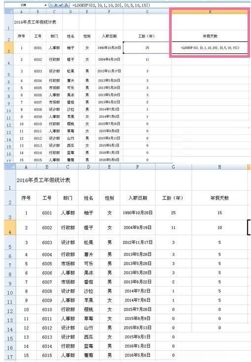
The first one is to enter [annual leave days" in cell H2 and the formula in cell H3: =LOOKUP(G3,{0,1,10,20} ,{0,5,10,15}), press [Enter/Enter] to calculate the number of annual leave days for employees. Among them, the LOOKUP function is to find matching conditions and fill in the corresponding data. The array {0,1,10,20} refers to the node data in the length of service, and the array {0,5,10,15} is the number of annual leave days under the corresponding length of service. Braces {} can be entered using shift [/shift]. Note that in English mode, or after entering the formula, press CTRL SHIFT ENTER to complete.

The second algorithm for annual leave days, enter the formula in cell H3: =IF(G3

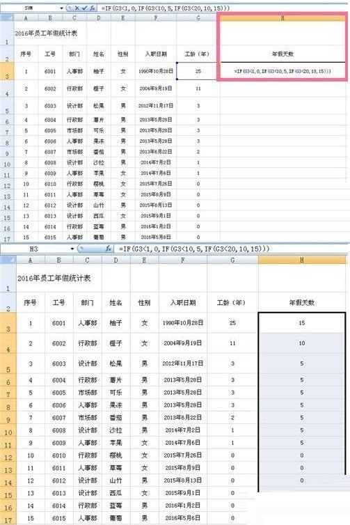
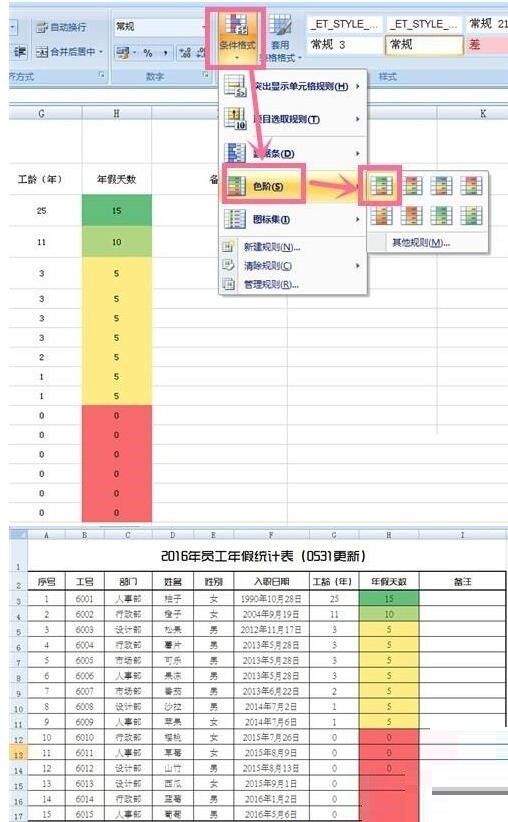
5. Finally, in order to highlight the difference in annual leave days, you can select a format through [Conditional Formatting]-[Data Bar]. Then, by adjusting the font and alignment, the entire table is completed.

Note:

The braces {} in the array can be entered using shift [ and shift ]. Note that in English mode, or after entering the formula, press CTRL SHIFT ENTER to complete.

The above is the detailed content of How to use the if multiple function in Excel to create employee annual leave table. For more information, please follow other related articles on the PHP Chinese website!