


php editor strawberry introduces you to the use of functions in excel documents. In excel, functions are very important tools that can help users quickly calculate data and analyze information. By using various functions, users can implement complex calculations, logical judgments, text processing and other operations. Proficient in using excel functions will help improve work efficiency and improve data processing capabilities. This article will introduce you to the classification, grammatical format and practical application skills of commonly used excel functions in detail, allowing you to easily master the key points of using excel functions.
1. For example, there are two tables: Table A and Table B.


The example requires that cells B26 to B31 of table B be automatically filled in with the same values in column A of table A and column A of table B (identical, not The value in column B corresponding to uppercase and lowercase).
2. First select B table B26, then select the formula and insert the vlookup function.

#3. The function editing box pops up, as shown in the figure.
Just fill in all the custom items. The first one from top to bottom is: You can use the mouse to directly select Table B A26. This is the search item to follow when returning to B26. The edit box will Automatically enter syntax. The second custom item is:
Directly select the entire A:B columns in table A with the mouse, which is the search range. If you want to circle a specific range, it is recommended to use $ to limit it to prevent errors when copying the formula later.
The third one is: In this example, the value to be returned is in column 2 of the search range circled above, so just enter the number 2.
The last one: Exact matching is usually required, so FALSE should be filled in. You can also directly type in the number 0, which has the same meaning.

4. After confirmation, you can see the return value in B26 of table B:

5. Finally, Just copy the formula down.

The above is the detailed content of How to use functions in excel documents. For more information, please follow other related articles on the PHP Chinese website!

 How to Format a Spilled Array in ExcelApr 10, 2025 pm 12:01 PM
Use formula conditional formatting to handle overflow arrays in Excel Direct formatting of overflow arrays in Excel can cause problems, especially when the data shape or size changes. Formula-based conditional formatting rules allow automatic formatting to be adjusted when data parameters change. Adding a dollar sign ($) before a column reference applies a rule to all rows in the data. In Excel, you can apply direct formatting to the values or background of a cell to make the spreadsheet easier to read. However, when an Excel formula returns a set of values (called overflow arrays), applying direct formatting will cause problems if the size or shape of the data changes. Suppose you have this spreadsheet with overflow results from the PIVOTBY formula,
 You Need to Know What the Hash Sign Does in Excel FormulasApr 08, 2025 am 12:55 AM
Excel Overflow Range Operator (#) enables formulas to be automatically adjusted to accommodate changes in overflow range size. This feature is only available for Microsoft 365 Excel for Windows or Mac. Common functions such as UNIQUE, COUNTIF, and SORTBY can be used in conjunction with overflow range operators to generate dynamic sortable lists. The pound sign (#) in the Excel formula is also called the overflow range operator, which instructs the program to consider all results in the overflow range. Therefore, even if the overflow range increases or decreases, the formula containing # will automatically reflect this change. How to list and sort unique values in Microsoft Excel
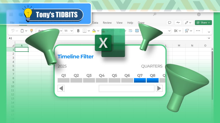 How to Create a Timeline Filter in ExcelApr 03, 2025 am 03:51 AM
In Excel, using the timeline filter can display data by time period more efficiently, which is more convenient than using the filter button. The Timeline is a dynamic filtering option that allows you to quickly display data for a single date, month, quarter, or year. Step 1: Convert data to pivot table First, convert the original Excel data into a pivot table. Select any cell in the data table (formatted or not) and click PivotTable on the Insert tab of the ribbon. Related: How to Create Pivot Tables in Microsoft Excel Don't be intimidated by the pivot table! We will teach you basic skills that you can master in minutes. Related Articles In the dialog box, make sure the entire data range is selected (
 How to Use the GROUPBY Function in ExcelApr 02, 2025 am 03:51 AM
Excel's GROUPBY function: Powerful data grouping and aggregation tools Excel's GROUPBY function allows you to group and aggregate data based on specific fields in a data table. It also provides parameters that allow you to sort and filter the data so that you can customize the output to your specific needs. GROUPBY function syntax The GROUPBY function contains eight parameters: =GROUPBY(a,b,c,d,e,f,g,h) Parameters a to c are required: a (row field): A range (one column or multiple columns) containing the value or category to which the data is grouped. b (value): The range of values containing aggregated data (one column or multiple columns).
 Don't Hide and Unhide Columns in Excel—Use Groups InsteadApr 01, 2025 am 12:38 AM
Excel efficient grouping: say goodbye to hidden columns and embrace flexible data management! While hidden columns can temporarily remove unnecessary data, grouping columns are often a better choice when dealing with large data sets or pursuing flexibility. This article will explain in detail the advantages and operation methods of Excel column grouping to help you improve data management efficiency. Why is grouping better than hiding? Hiding columns (right-click on the column title and select "Hide") can easily lead to data forgetting, even the column title prompt is not reliable because the title itself can be deleted. In contrast, grouped columns are faster and more convenient to expand and fold, which not only improves work efficiency, but also enhances user experience, especially when multi-person collaboration. Additionally, grouping columns allow creation of subgroups, which cannot be achieved by hidden columns. This is the number
 How to Completely Hide an Excel WorksheetMar 31, 2025 pm 01:40 PM
Excel worksheets have three levels of visibility: visible, hidden, and very hidden. Setting the worksheet to "very hidden" reduces the likelihood that others can access them. To set the worksheet to "very hidden", set its visibility to "xlsSheetVeryHidden" in the VBA window. Excel worksheets have three levels of visibility: visible, hidden, and very hidden. Many people know how to hide and unhide the worksheet by right-clicking on the tab area at the bottom of the workbook, but this is just a medium way to remove the Excel worksheet from the view. Whether you want to organize the workbook tabs, set up dedicated worksheets for drop-down list options and other controls, keeping only the most important worksheets visible, and
 Use the PERCENTOF Function to Simplify Percentage Calculations in ExcelMar 27, 2025 am 03:03 AM
Excel's PERCENTOF function: Easily calculate the proportion of data subsets Excel's PERCENTOF function can quickly calculate the proportion of data subsets in the entire data set, avoiding the hassle of creating complex formulas. PERCENTOF function syntax The PERCENTOF function has two parameters: =PERCENTOF(a,b) in: a (required) is a subset of data that forms part of the entire data set; b (required) is the entire dataset. In other words, the PERCENTOF function calculates the percentage of the subset a to the total dataset b. Calculate the proportion of individual values using PERCENTOF The easiest way to use the PERCENTOF function is to calculate the single
 If You Don't Use Excel's Hidden Camera Tool, You're Missing a TrickMar 25, 2025 am 02:48 AM
Quick Links Why Use the Camera Tool?


Hot AI Tools

Undresser.AI Undress
AI-powered app for creating realistic nude photos

AI Clothes Remover
Online AI tool for removing clothes from photos.

Undress AI Tool
Undress images for free

Clothoff.io
AI clothes remover

AI Hentai Generator
Generate AI Hentai for free.

Hot Article
Hot Tools

Dreamweaver CS6
Visual web development tools

DVWA
Damn Vulnerable Web App (DVWA) is a PHP/MySQL web application that is very vulnerable. Its main goals are to be an aid for security professionals to test their skills and tools in a legal environment, to help web developers better understand the process of securing web applications, and to help teachers/students teach/learn in a classroom environment Web application security. The goal of DVWA is to practice some of the most common web vulnerabilities through a simple and straightforward interface, with varying degrees of difficulty. Please note that this software

SAP NetWeaver Server Adapter for Eclipse
Integrate Eclipse with SAP NetWeaver application server.

Zend Studio 13.0.1
Powerful PHP integrated development environment

ZendStudio 13.5.1 Mac
Powerful PHP integrated development environment

