Quantitative model of parallel computing and its application in deep learning engine

UI. How to train deep learning models faster has been the focus of the industry. Industry players either develop special hardware or develop software frameworks, each showing their unique abilities.

Of course, these laws can be seen in computer architecture textbooks and literature, such as this "Computer Architecture: a Quantative Approach", but the value of this article lies in Select the most fundamental laws in a targeted manner and combine them with a deep learning engine to understand them.

1 Assumptions about the amount of calculation

Before studying the quantitative model of parallel computing, we first make some settings. For a specific deep learning model training task, assuming that the total calculation amount V is fixed, it can be roughly considered that as long as the calculation of the magnitude of V is completed, the deep learning model will complete the training.

This GitHub page (https://github.com/albanie/convnet-burden) lists the calculation amount required by common CNN models to process an image. It should be noted that what is listed on this page is The amount of calculation in the forward phase requires calculation in the backward phase during the training phase. Usually, the amount of calculation in the backward phase is greater than the amount of forward calculation. This paper (https://openreview.net/pdf?id=Bygq-H9eg) gives an intuitive visualization result of the calculation amount of processing an image in the training stage:

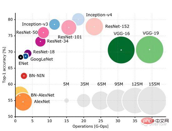
Taking ResNet-50 as an example, the training phase requires 8G-Ops (about 8 billion calculations) to process a 224X224x3 image. The entire ImageNet data set has approximately 1.2 million images. The training process requires processing 90 of the entire data set. Epochs, a rough estimate, the training process requires a total of (8*10^9) *(1.2*10^6)* 90 = 0.864*10^18 operations, then the total calculation amount of the ResNet-50 training process is approximately One billion times one billion operations, we can simply think that as long as these calculations are completed, the model operation is completed. The goal of the deep learning computing engine is to complete this given amount of calculation in the shortest time.

2 Assumptions about computing devices

This article is limited to the processor-centric computing device (Processor-centric computing) shown in the figure below, and the memory-centric computing (Processing in memory) devices are being explored in the industry, but they are not yet mainstream.

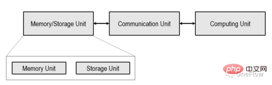
The Computing Unit in the computing device shown in the above figure can be a general-purpose processor such as CPU, GPGPU, or a special-purpose chip such as TPU. If the Computing Unit is a general-purpose chip, usually programs and data are stored in the Memory Unit, which is also the most popular von Neumann structure computer today.

If the Computing Unit is a dedicated chip, usually only data is stored in the Memory Unit. The Communication Unit is responsible for transferring data from the Memory Unit to the Computing Unit and completing the data loading. After the Computing Unit gets the data, it is responsible for completing the calculation (form conversion of the data). The Communication Unit then transfers the calculation results to the Memory Unit to complete the data storage. (Store).

The transmission capability of the Communication Unit is usually expressed by the memory access bandwidth beta, that is, the number of bytes that can be transported per second, which is usually related to the number of cables and the frequency of the signal. The computing power of a Computing Unit is usually represented by the throughput rate pi, which is the number of floating-point calculations (flops) that can be completed per second. This is usually related to the number of logical computing devices integrated on the computing unit and the clock frequency.

The goal of the deep learning engine is to maximize the data processing capabilities of the computing device through software and hardware co-design, that is, to complete a given amount of calculations in the shortest time.

3 Roofline Model: A mathematical model that depicts actual computing performance

The actual computing performance (number of operations completed per second) that a computing device can achieve when executing a task is not only related to the memory access bandwidth Beta is related to the theoretical peak pi of the computing unit, and also to the operational intensity (Arithemetic intensity, or Operational intensity) of the current task itself.

The operation intensity of a task is defined as the number of floating point calculations required for each byte of data, that is, Flops per byte. Popularly understood, a task with low computational intensity means that the Computing Unit needs to perform fewer operations on a byte transported by the Communication Unit. In order to keep the Computing Unit busy in this case, the Communication Unit must frequently transport data;

A task with high computational intensity means that the Computing Unit needs to perform more operations on a byte transferred by the Communication Unit. The Communication Unit does not need to transfer data so frequently to keep the Computing Unit busy.

First of all, the actual computing performance will not exceed the theoretical peak pi of the computing unit. Secondly, if the memory access bandwidth beta is very small, only beta bytes can be transferred from the memory to the Computing Unit in 1 second. Let I represent the number of operations required for each byte in the current computing task, then beta * I represents 1 second. The actual number of operations required to transfer data within a clock. If beta * I

Roofline model is a mathematical model that infers actual computing performance based on the relationship between the memory access bandwidth, the peak throughput rate of the computing unit, and the computing intensity of the task. Published by David Patterson's team on Communications of ACM in 2008 ( https://en.wikipedia.org/wiki/Roofline_model ), it is a simple and elegant visual model:

Figure 1: Roofline Model

The independent variables on the horizontal axis of Figure 1 represent the computing intensity of different tasks, that is, the number of floating point operations required per byte. The dependent variable on the vertical axis represents the actual achievable computing performance, that is, the number of floating point operations performed per second. The above figure shows the actual computing performance that can be achieved by two tasks with computing intensity I_1 and I_2. The computing intensity of I_1 is less than pi/beta, which is called a memory access limited task. The actual computing performance beta * I_1 is lower than the theoretical peak pi .

The computing intensity of I_2 is higher than pi/beta, which is called a computing-limited task. The actual computing performance reaches the theoretical peak pi, and the memory access bandwidth only utilizes pi/(I_2*beta). The slope of the slope in the figure is beta. The intersection of the slope and the theoretical peak pi horizontal line is called the ridge point. The abscissa of the ridge point is pi/beta. When the computing intensity of the task is equal to pi/beta, the Communication Unit It is in a balanced state with the Computing Unit, and neither one is wasted.

Recalling that the goal of the deep learning engine is to "complete a given amount of calculations in the shortest time", it is necessary to maximize the actual achievable computing performance of the system. To achieve this goal, several strategies are available.

I_2 in Figure 1 is a computing-limited task. Actual computing performance can be improved by increasing the parallelism of the Computing Unit and thereby increasing the theoretical peak value. For example, integrating more computing logic units on the Computing Unit ( ALU). Specific to deep learning scenarios, it means adding GPUs, from one GPU to several GPUs operating at the same time.

As shown in Figure 2, when more parallelism is added to the Computing Unit, the theoretical peak value is higher than beta * I_2, then the actual computing performance of I_2 is higher, and it only takes a shorter time. Can.

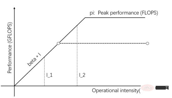
Figure 2: Increase the theoretical peak value of Computing Unit to improve actual computing performance

I_1 in Figure 1 is a memory access-limited task, then Actual computing performance and data supply capabilities can be improved by improving the transmission bandwidth of the Communication Unit. As shown in Figure 3, the slope of the slope represents the transmission bandwidth of the Communication Unit. When the slope of the slope increases, I_1 changes from a memory access-limited task to a calculation-limited task, and the actual computing performance is improved.

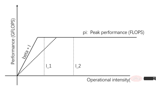
Figure 3: Improving the data supply capability of the Communication Unit to improve actual computing performance

In addition to improving the actual computing performance by improving the transmission bandwidth or theoretical peak of the hardware In addition to performance, actual computing performance can also be improved by improving the computing intensity of the task itself. The same task can be implemented in many different ways, and the computing intensity of different implementations also differs. After the computing intensity is transformed from I_1 to exceed pi/beta, it becomes a computing-limited task, and the actual computing performance reaches pi, exceeding the original beta*I_1.

In actual deep learning engines, the above three methods (increasing parallelism, improving transmission bandwidth, and using algorithms with better computational intensity) are all used.

4 Amdahl's Law: How to calculate speedup ratio?

The example in Figure 2 improves actual computing performance by increasing the parallelism of the Computing Unit. How much can the execution time of the task be shortened? This is the issue of acceleration ratio, that is, the efficiency is increased several times.

For the convenience of discussion, (1) We assume that the current task is computationally limited, let I represent the computing intensity, that is, I*beta>pi. After increasing the computing unit of the Computing Unit by s times, the theoretical calculation peak is s * pi. Assume that the computing intensity I of the task is high enough so that after the theoretical peak value is increased by s times, it is still computationally limited, that is, I*beta > s*pi; (2) Assuming that no pipeline is used, the Communication Unit and Computing Unit are always executed sequentially (we will discuss the impact of the pipeline specifically later). Let's calculate how many times the task execution efficiency has improved.

In the initial situation where the theoretical peak value is pi, the Communication Unit transfers beta bytes of data in 1 second, and the Computing Unit needs (I*beta)/pi seconds to complete the calculation. That is, if the calculation of I*beta is completed within 1 (I*beta)/pi second, then the calculation of (I*beta) / (1 (I*beta)/pi) can be completed per unit time, assuming the total calculation amount is V, then it takes t1=V*(1 (I*beta)/pi)/(I*beta) seconds in total.

After increasing the theoretical calculation peak by s times by increasing the parallelism, the Communication Unit still needs 1 second to transfer beta bytes of data, and the Computing Unit needs (I*beta)/(s*pi) seconds to complete. calculate. Assuming that the total calculation amount is V, it takes t2=V*(1 (I*beta)/(s*pi))/(I*beta) seconds to complete the task.

Calculate t1/t2 to get the acceleration ratio: 1/(pi/(pi I*beta) (I*beta)/(s*(pi I*beta))). I’m sorry that this formula is ugly. Readers can It's relatively simple to deduce it yourself.

When the theoretical peak value is pi, it takes 1 second to transfer data and (I*beta)/pi seconds to calculate. Then the proportion of calculation time is (I*beta)/(pi I*beta ), we let p represent this ratio, equal to (I*beta)/(pi I*beta).

Substituting p into the acceleration ratio of t1/t2, we can get the acceleration ratio as 1/(1-p p/s). This is the famous Amdahl's law (https://en.wikipedia.org/wiki/ Amdahl's_law). Where p represents the proportion of the original task that can be parallelized, s represents the multiple of parallelization, and 1/(1-p p/s) represents the speedup obtained.

Let us use a simple number to calculate. Assume that the Communication Unit takes 1 second to transfer data and the Computing Unit takes 9 seconds to calculate, then p=0.9. Assume that we enhance the parallelism of the Computing Unit and increase its theoretical peak value by 3 times, that is, s=3. Then the Computing Unit only takes 3 seconds to complete the calculation. So what is the acceleration ratio? Using Amdahl's law, we can know that the acceleration ratio is 2.5 times, and the acceleration ratio 2.5 is less than the parallelism multiple of 3 of the Computing Unit.

We have tasted the sweetness of increasing the parallelism of the Computing Unit. Can we obtain a better acceleration ratio by further increasing the parallelism s? Can. For example, if s=9, then we can obtain a 5x acceleration ratio, and we can see that the benefits of increasing parallelism are getting smaller and smaller.

Can we increase the speedup ratio by increasing s infinitely? Yes, but it is becoming less and less cost-effective. Just imagine that if s tends to infinity (that is, if the theoretical peak value of the Computing Unit is infinite), p/s will tend to 0, then the maximum acceleration ratio is 1/(1-p)=10.

As long as there is a non-parallelizable part (Communication Unit) in the system, the acceleration ratio cannot exceed 1/(1-p).

The actual situation may be worse than the upper limit of acceleration ratio 1/(1-p), because the above analysis assumes that the computing intensity I is infinite, and when increasing the parallelism of the Computing Unit, it will usually make the Communication Unit As the transmission bandwidth decreases, p becomes smaller and 1/(1-p) becomes larger.

This conclusion is very pessimistic. Even if the communication overhead (1-p) only accounts for 0.01, it means that no matter how many parallel units are used, tens of thousands, we can only obtain a maximum speedup of 100 times. Is there any way to make p as close to 1 as possible, that is, 1-p approaches 0, thereby improving the acceleration ratio? There’s a magic bullet: the assembly line.

5 Pipelining: Panacea

When deriving Amdahl's law, we assumed that the Communication Unit and the Computing Unit work in series. The Communication Unit always carries data first, and the Computing Unit does calculations. After completion, the Communication Unit is asked to transfer the data, and then calculate again, and so on.

Can the Communication Unit and Computing Unit work at the same time, transferring data and calculating at the same time? If the Computing Unit can immediately start calculating the next batch of data after calculating a piece of data, then p will be almost 1. No matter how many times the parallelism degree s is increased, a linear acceleration ratio can be obtained. Let's examine the conditions under which linear speedup can be obtained.

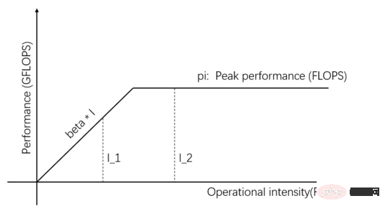
Figure 4: (Same as Figure 1) Roofline Model

I_1 in Figure 4 is a communication-limited task, and the Communication Unit can handle it in 1 second For beta-byte data, the amount of calculation required by the Computing Unit to process this beta-byte is beta*I_1 operations. The theoretical calculation peak is pi, and a total of (beta*I_1)/pi seconds is needed to complete the calculation.

For communication-limited tasks, we have beta*I_1

I_2 in Figure 4 is a computationally limited task. The Communication Unit can transfer beta bytes of data in 1 second. The amount of calculation required by the Computing Unit to process these beta bytes is beta*I_2 operations. Theoretical calculation The peak value is pi, and it takes (beta*I_2)/pi seconds to complete the calculation. For computing-limited tasks, we have beta*I_2>pi, so the computing time of the Computing Unit is greater than 1 second.

This also means that it takes several seconds to complete the calculation of the data that takes 1 second to transfer. There is enough time to transfer the next batch of data within the calculation time, that is, the calculation time can be covered up. In terms of data transfer time, p is at most 1. As long as I is infinite, the acceleration ratio can be infinite.

The technology that enables the Communication Unit and Computing Unit to overlap is called pipelining (Pipeling: https://en.wikipedia.org/wiki/Pipeline_(computing) ). It is a technology that effectively improves Computing Unit utilization and improves acceleration ratio.

6 The inspiration of the quantitative model of parallel computing for deep learning engines

The various quantitative models discussed above are also applicable to the development of deep learning engines. For example, for computing-limited tasks, you can increase the degree of parallelism (increase graphics card) to accelerate; even if the same hardware device is used, using different parallel methods (data parallelism, model parallelism or pipeline parallelism) will affect the computing intensity I, thus affecting the actual computing performance; the distributed deep learning engine contains a large number of Communication overhead and runtime overhead, how to reduce or mask these overheads is crucial to the acceleration effect.

Understanding the deep learning model based on GPU training from the perspective of a Processor-centric computing device, readers can think about how to design a deep learning engine to obtain a better acceleration ratio.

In the case of a single machine and a single card, 100% utilization of the GPU can be achieved only by completing the data transfer and calculation pipeline. The actual computing performance ultimately depends on the efficiency of the underlying matrix calculation, that is, the efficiency of cudnn. In theory, there should be no performance gap between various deep learning frameworks in a single-card scenario.

If you want to gain acceleration by adding GPUs within the same machine, compared with the single-card scenario, it increases the complexity of data transfer between GPUs and different tasks. The segmentation method may produce different computing intensity I (for example, the convolutional layer is suitable for data parallelism, and the fully connected layer is suitable for model parallelism). In addition to communication overhead, runtime scheduling overhead also affects the speedup.

In multi-machine and multi-card scenarios, the complexity of data transfer between GPUs is further increased. The bandwidth of data transfer between machines through the network is generally lower than that of data transfer within the machine through PCIe. bandwidth, which means that the degree of parallelism has increased, but the data transfer bandwidth has decreased, which means that the slope of the diagonal line in the Roofline model has become smaller. Scenarios such as CNN that are suitable for data parallelism usually mean relatively high computing intensity I, and There are also some models, such as RNN/LSTM, whose computational intensity I is much smaller, which also means that the communication overhead in the pipeline is more difficult to cover up.

7 Summary

Readers who have used distributed deep learning engines should have a personal experience of the acceleration ratio of the software framework. Basically, convolutional neural networks are suitable for data parallelism (computing intensity). For models with higher I), the effect of accelerating by adding GPU is quite satisfactory. However, there is a large class of neural networks that use model parallelism and have higher computational intensity. Moreover, even if model parallelism is used, the computational intensity is still very low. It is also far lower than convolutional neural networks. How to accelerate these applications by increasing GPU parallelism is an unsolved problem in the industry.

In previous deep learning evaluations, it even occurred that using multiple GPUs to train RNN was slower than a single GPU ( https://rare-technologies.com/machine-learning-hardware-benchmarks/ ). No matter what technology is used to solve the efficiency problem of the deep learning engine, it remains the same. In order to improve the acceleration ratio, it is all about reducing runtime overhead, choosing an appropriate parallel mode to increase computing intensity, and masking communication overhead through pipelines. Within the scope covered by the basic laws described in this article.

The above is the detailed content of Quantitative model of parallel computing and its application in deep learning engine. For more information, please follow other related articles on the PHP Chinese website!