Design and implementation of database anomaly monitoring system based on AI algorithm

Author: Cao Zhenweiyuan

The Meituan database platform R&D team is faced with the increasingly urgent need to discover database anomalies. In order to discover, locate and stop losses more quickly and intelligently, we have developed a database based on AI algorithms. Anomaly detection services.

1. Background

The database is widely used in Meituan’s core business scenarios, with high stability requirements and very low tolerance for exceptions. Therefore, rapid database anomaly discovery, location and stop loss become increasingly important. In response to the problem of abnormal monitoring, the traditional fixed threshold alarm method requires expert experience to configure rules, and cannot flexibly and dynamically adjust the threshold according to different business scenarios, which can easily turn small problems into major failures.

The AI-based database anomaly detection capability can conduct 7*24-hour inspections of key indicators based on the historical performance of the database, and can detect risks in the budding state of abnormalities earlier. It exposes abnormalities and assists R&D personnel in locating and stopping losses before the problem worsens. Based on the considerations of the above factors, the Meituan database platform R&D team decided to develop a database anomaly detection service system. Next, this article will elaborate on some of our thoughts and practices from several dimensions such as feature analysis, algorithm selection, model training and real-time detection.

2. Feature analysis

2.1 Find out the changing patterns of data

Before proceeding with specific development and coding, there is a very important task, which is From existing historical monitoring indicators, we can discover the changing patterns of time series data, and then select appropriate algorithms based on the characteristics of data distribution. The following are some representative indicator distribution charts we selected from historical data: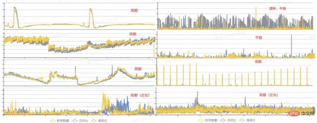

Figure 1 Database indicator form

From the above figure, we can see that the data patterns mainly present three states: cycle, drift and stationary^[1]. Therefore, we can model samples with these common characteristics in the early stage, which can cover most scenarios. Next, we analyze it from three perspectives: periodicity, drift and stationarity, and discuss the algorithm design process.

2.1.1 Cyclic changes

In many business scenarios, indicators will fluctuate regularly due to morning and evening peaks or some scheduled tasks. We believe that this is an inherent regular fluctuation of the data, and the model should have the ability to identify periodic components and detect contextual anomalies. For time series indicators that do not have a long-term trend component, when the indicator has a cyclical component, , where T represents the period span of the time series. The autocorrelation diagram can be calculated, that is, the value of when t takes different values, and then the periodicity can be determined by analyzing the interval of the autocorrelation peak. The main process includes the following steps:

1. Extract trend components and separate the residual sequence. Use the moving average method to extract the long-term trend term, and make the difference with the original sequence to obtain the residual sequence (The periodic analysis here has nothing to do with the trend. If the trend component is not separated, the autocorrelation will be significantly affected. , it is difficult to identify the period ).
2. Calculate the cyclic autocorrelation (Rolling Correlation) sequence of the residuals. The autocorrelation sequence is calculated by performing a vector dot multiplication operation with the residual sequence after cyclically moving the residual sequence (Cyclic autocorrelation can avoid delayed attenuation).
3. Determine the period T based on the peak coordinates of the autocorrelation sequence. Extract a series of local highest peaks of the autocorrelation sequence, and take the interval of the abscissa as the period (If the autocorrelation value corresponding to the periodic point is less than the given threshold, it is considered to have no significant periodicity).

The specific process is as follows:

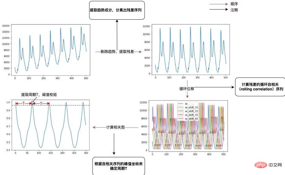
Figure 2 Schematic of the cycle extraction process

2.1.2 Drift changes

For the model to be modeled Sequence is usually required to have no obvious long-term trend or global drift, otherwise the generated model usually cannot adapt well to the latest trend of the indicator^[2]. We refer to situations where the mean value of a time series changes significantly over time or there is a global mutation point, collectively referred to as a drift scenario. In order to accurately capture the latest trend of the time series, we need to determine whether there is drift in the historical data in the early stage of modeling. Global drift and periodic series mean drift, as shown in the following example:

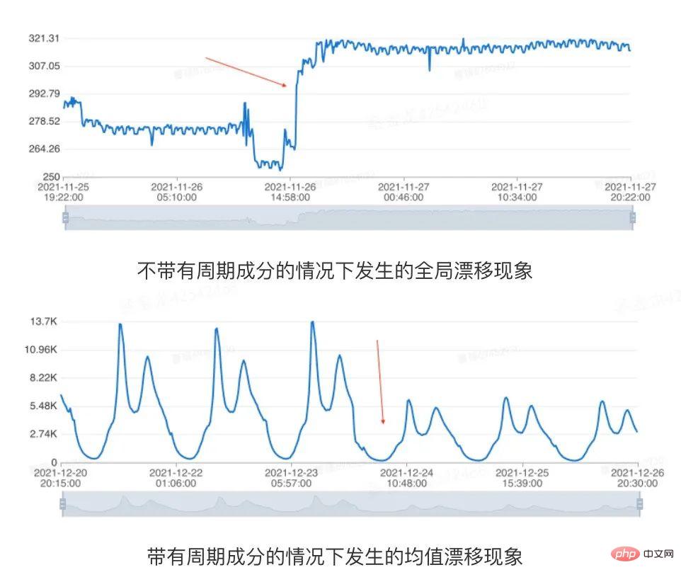
Figure 3 Data drift diagram

Database indicators are affected by complex factors such as business activities. Many data will have non-periodic changes, and modeling needs to tolerate these changes. Therefore, different from the classic change point detection problem, in the anomaly detection scenario, we only need to detect the situation where the data is stable in history and then drifts. Based on the algorithm performance and actual performance, we used the drift detection method based on median filtering. The main process includes the following links:

1. Median smoothing

# a. According to the size of the given window, extract the median within the window to obtain the trend component of the time series.

b. The window needs to be large enough to avoid the influence of periodic factors and perform filter delay correction.

c. The reason for using median rather than mean smoothing is to avoid the influence of abnormal samples.

2. Determine whether the smoothed sequence is increasing or decreasing

#a. Serial data after median smoothing , if each point is greater than ( is less than ) the previous point, the sequence is an increasing (decreasing) sequence.

b. If the sequence is strictly increasing or strictly decreasing, then the indicator obviously has a long-term trend, and it can be terminated early.

3. Traverse the smooth sequence and use the following two rules to determine whether there is drift

a. If the maximum value of the sequence to the left of the current sample point is less than the minimum value of the sequence to the right of the current sample point, there is a sudden drift (Uptrend).

b. If the minimum value of the sequence to the left of the current sample point is greater than the maximum value of the sequence to the right of the current sample point, there is a sudden drop drift (Downtrend).

2.1.3 Stationary changes

For a time series indicator, if its properties do not change with the change of observation time at any moment, we believe that this The time series is stable. Therefore, for time series with long-term trend components or cyclical components, they are all non-stationary. The specific example is shown in the figure below:

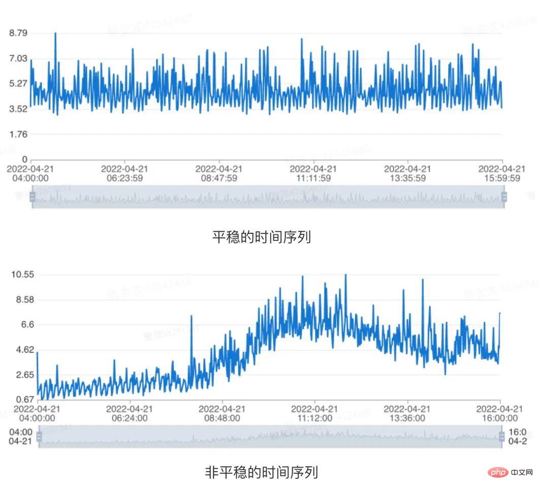
Figure 4 Data stability indication

In view of this situation, We can determine whether a given time series is stationary through the unit root test (Augmented Dickey-Fuller Test)^[3]. Specifically, for a piece of historical data of a given time range indicator, we believe that the time series is stable when the following conditions are met at the same time:

1. The p-value obtained by adfuller test for the time series data of the last 1 day is less than 0.05.
2. The p-value obtained by adfuller test for the time series data of the last 7 days is less than 0.05.

3. Algorithm selection

3.1 Distribution rules and algorithm selection

By understanding the performance of some well-known companies in the industry in time series data anomaly detection According to the product introduction published on the Internet, coupled with our accumulated historical experience and sampling analysis of some actual online indicators, their probability density functions conform to the following distribution:

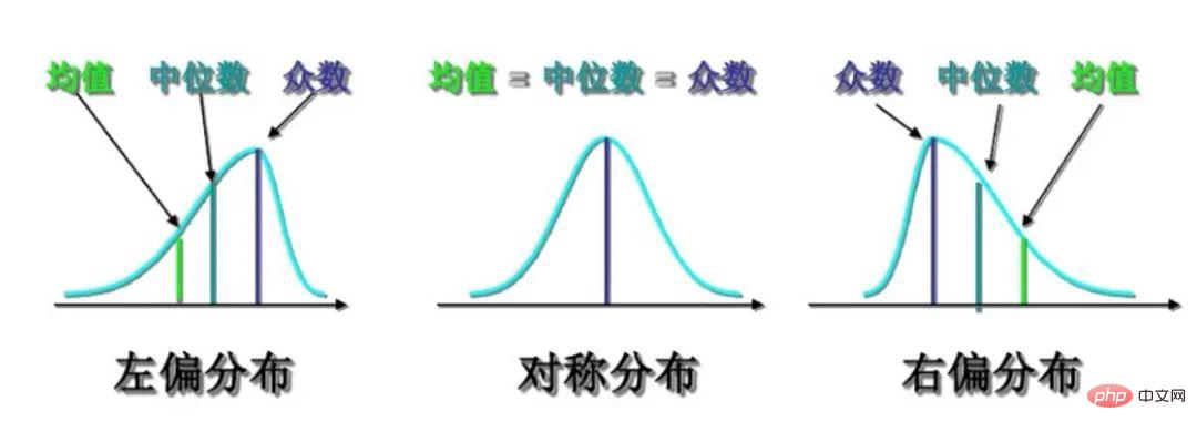
Figure 5 Distribution skewness representation

For the above distribution, we investigated some common algorithms and determined the box plot, absolute median difference and Extreme value theory as the ultimate anomaly detection algorithm. The following is a comparison table of algorithms for common time series data detection:

The main reason why we did not choose 3Sigma is that it has low tolerance for anomalies, while In theory, the absolute median difference has better tolerance for abnormalities, so when the data presents a highly symmetric distribution, the absolute median difference (MAD) is used instead of 3Sigma for detection. We use different detection algorithms for different data distributions (For the principles of different algorithms, please refer to the appendix at the end of the article, I will not elaborate too much here):

1. Low skewness and high symmetry distribution: Median absolute difference (MAD)
2. Medium skewness Distribution: Box plot (Boxplot)
3. Highly skewed distribution: Extreme value theory (EVT)

With the above analysis, we can get the specific process of outputting the model based on the sample:

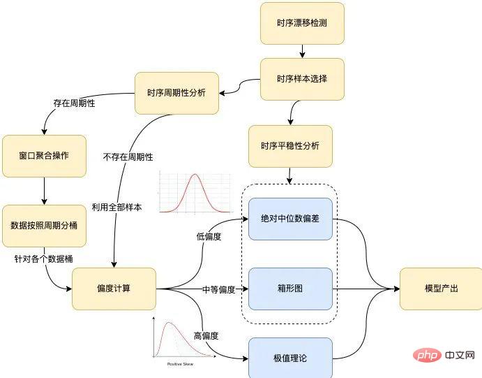
Figure 6 Algorithm modeling process

The overall modeling process of the algorithm is shown in the figure above, which mainly covers the following branches: timing drift detection, timing stability sexual analysis, time series periodicity analysis and skewness calculation. The following are introduced respectively:

1. Timing drift detection. If the scene where drift exists is detected, the input time series needs to be cut according to the drift point t obtained by the detection, and the time series samples after the drift point are used as the input of the subsequent modeling process, recorded as S={Si}, where i>t.
2. Time series stationarity analysis. If the input time series S satisfies the stationarity test, modeling will be performed directly through the box plot (default) or the absolute median difference.
3. Timing periodicity analysis. In the case of periodicity, the period span is recorded as T, the input time series S is cut according to the span T, and the modeling process is carried out for the data bucket composed of each time index j∈{0,1,⋯,T−1} . In the absence of periodicity, the modeling process is performed for all input time series S as data buckets.

Case : Given a time series ts={t₀,t₁,⋯ ,t_n}, assuming that there is periodicity and the period span is T, for the time index j, where j∈{0,1,⋯,T−1}, it is necessary to model it The sample points are composed of the interval [t_j−kT−m, t_{j−kT m}], where m is a parameter, representing the window size, and k is an integer, satisfying j−kT −m≥0, j−kT m≤n. For example, assuming that the given time series starts from 2022/03/01 00:00:00 to 2022/03/08 00:00:00, the given window size is 5, and the period span is one day, then for the time index 30 In other words, the sample points required to model it will come from the following time period: [03/01 00:25:00, 03/01 00:35:00]
[03/02 00:25:00, 03/02 00:35:00]
...
[03/07 00:25:00, 03/07 00:35:00]

4. skewness calculation. The time series indicators are converted into probability distribution diagrams, and the skewness of the distribution is calculated. If the absolute value of the skewness exceeds the threshold, the extreme value theory is used to model the output threshold. If the absolute value of the skewness is less than the threshold, the threshold is modeled and output by box plot or absolute median difference.

3.2 Case Sample Modeling

A case is selected here to show the data analysis and modeling process to facilitate a clearer understanding of the above process. Figure (a) is the original sequence, Figure (b) is the sequence folded according to the span of days, Figure (c) is the amplified trend performance of the samples in a certain time index interval in Figure (b), Figure (d) ) is the lower threshold corresponding to the time index in figure (c). The following is a case of modeling historical samples of a certain time series:

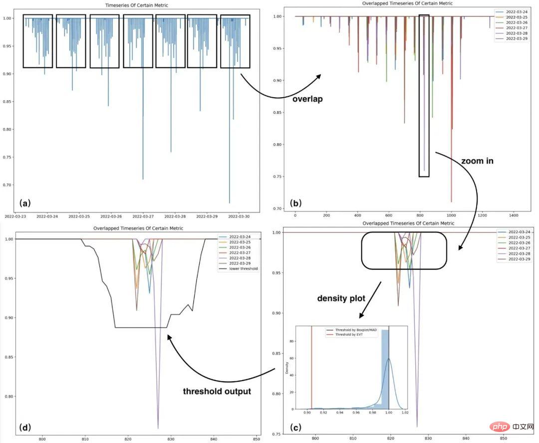
Figure 7 Modeling case

The sample distribution histogram and threshold in the area (c) of the above figure (Some abnormal samples have been eliminated), it can be seen that in this highly skewed distribution scenario, the threshold calculated by the EVT algorithm is more To be reasonable.

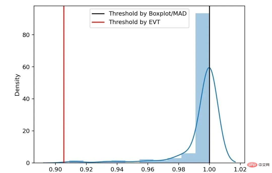
Figure 8 Skewed distribution threshold comparison

4. Model training and real-time detection

4.1 Data flow process

In order to detect large-scale second-level data in real time, we started from real-time stream processing based on Flink and designed the following technical solution:

1. Real-time detection part: Based on Flink real-time stream processing, consuming Mafka (Meituan’s internal message queue component ) messages are detected online, the results are stored in Elasticsearch (hereinafter referred to as ES), and exception records are generated.
2. Offline training part: Use Squirrel (Meituan’s internal KV database) as the task queue, from MOD (Meituan Internal operation and maintenance data warehouse) reads training data, reads parameters from the configuration table, trains the model, and saves it in ES. It supports automatic and manual triggering of training, and loads and updates the model by regularly reading the model library.

The following is the specific offline training and online detection technology design:

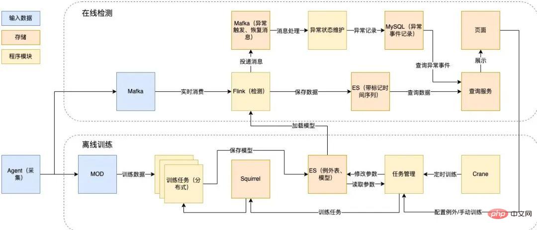
Figure 9 Offline training and online detection technology design

4.2 Anomaly detection process

The anomaly detection algorithm adopts the divide-and-conquer idea as a whole. In the model training stage, features are extracted based on historical data identification. Select an appropriate detection algorithm. This is divided into two parts: offline training and online detection. Offline mainly performs data preprocessing, time series classification and time series modeling based on historical conditions. Online mainly loads and uses offline trained models for online real-time anomaly detection. The specific design is shown in the figure below:

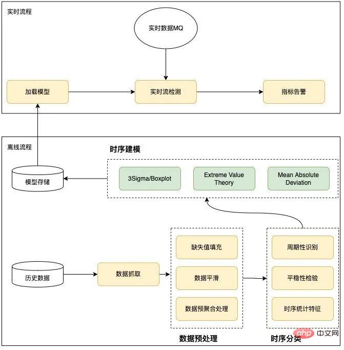
Figure 10 Anomaly detection process

5. Product Operation

In order to improve the efficiency of the optimization iterative algorithm and continue operations to improve precision and recall, we use Horae (Meituan’s internal scalable time series data anomaly detection system )’s case review capabilities enable a closed loop of online detection, case preservation, analysis and optimization, result evaluation, and online release.

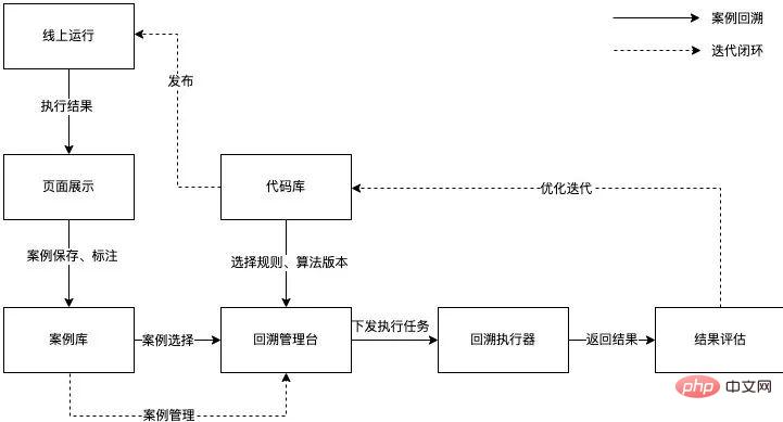
Figure 11 Operation process

Currently, the anomaly detection algorithm indicators are as follows ：

• Accuracy rate: Randomly select a part of cases where abnormalities are detected, and manually verify the proportion of cases that are indeed abnormal. is 81%.
• Recall rate: Based on faults, alarms and other sources, review the abnormal conditions of each indicator of the corresponding instance, and calculate the recall rate based on the monitoring results, as 82%.
• F1-score: The harmonic mean of precision and recall, which is 81%.

6. Future Outlook

Currently, Meituan’s database anomaly monitoring capabilities have been basically completed, and we will continue to work on the product in the future. Optimize and expand, specific directions include:

1. Have the ability to identify exception types. It can detect abnormal types, such as mean changes, fluctuation changes, spikes, etc., supports alarm subscription according to abnormal types, and inputs them as features into the subsequent diagnosis system, improving the database autonomy ecosystem^[4] .
2. Building Human-in-Loop environment. Support automatic learning based on feedback annotation, ensure continuous optimization of the model^[5].
3. Support for multiple database scenarios. The anomaly detection capability is platform-based to support more database scenarios, such as DB end-to-end error reporting, node network monitoring, etc.

7. Appendix

7.1 Absolute median difference

Absolute median difference, that is, Median Absolute Deviation(MAD), is a robust measure of sample deviation of univariate numerical data ^[6], usually calculated by the following formula:

When the prior is normal distribution, generally C chooses 1.4826 and k chooses 3. MAD assumes that the middle 50% of the samples are normal samples, while the abnormal samples fall within the 50% areas on both sides. When the sample obeys the normal distribution, the MAD indicator is better able to adapt to outliers in the data set than the standard deviation. For the standard deviation, the square of the distance from the data to the mean is used. The larger the deviation, the greater the weight. The impact of outliers on the results cannot be ignored. For MAD, a small amount of outliers will not affect the results of the experiment. The MAD algorithm does not affect the data. There are higher requirements for normality.

7.2 Box plot

The box plot mainly describes the discreteness and symmetry of the sample distribution through several statistics, including:

• Q0: Minimum value (Minimum)
• ##Q1: Lower quartile (Lower Quartile )
• Q2: Median (Median)
• Q3: Upper quartile ( Upper Quartile)
• Q4: Maximum value (Maximum)

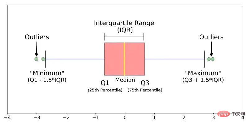
Figure 12 Box plot

Compare Q1 with Q## The distance between #3 _{is called IQR. When the sample deviates from the IQR of 1.5 times the upper quartile (} or deviates from the IQR of 1.5 times the lower quartile) , treating the sample as an outlier. Unlike three standard deviations based on the normality assumption, box plots generally do not make any assumptions about the underlying data distribution of the sample, can describe the discrete situation of the sample, and have a higher confidence in the potential abnormal samples contained in the sample. Tolerance. For biased data, Boxplot’s calibrated modeling is more consistent with the data distribution[7]^. 7.3 Extreme Value Theory

Real-world data is difficult to generalize with a known distribution, for example, for some extreme events (

anomalous), probability models (such as Gaussian distribution) often give its probability of 0. Extreme value theory[8] is to infer the distribution of extreme events that we may observe without any distribution assumptions based on the original data. This is the extreme value distribution (^EVD ). Its mathematical expression is as follows (Complementary cumulative distribution function formula):

where t represents the empirical threshold of the sample. Different values ​​can be set for different scenarios, which are the shape parameters and scale parameters in the generalized Pareto distribution. When a given sample exceeds the artificially set empirical threshold In the case of t, the random variable X-t obeys the generalized Pareto distribution. Through the maximum likelihood estimation method, we can calculate the parameter estimates and , and obtain the model threshold through the following formula:

In the above formula q represents the risk parameter, n is the number of all samples, and Nt is the number of samples that satisfy x-t>0. Since there is usually no a priori information for estimating the empirical threshold t, the sample empirical quantile can be used to replace the numerical value t. The value of the empirical quantile here can be selected according to the actual situation.

8. References

[1] Ren, H., Xu, B., Wang, Y., Yi, C., Huang, C., Kou, X., ... & Zhang, Q. (2019, July). Time-series anomaly detection service at microsoft. In Proceedings of the 25th ACM SIGKDD international conference on knowledge discovery & data mining (pp. 3009-3017) .

[2] Lu, J., Liu, A., Dong, F., Gu, F., Gama, J., & Zhang, G. (2018). Learning under concept drift: A review. IEEE Transactions on Knowledge and Data Engineering, 31(12), 2346-2363.

[3] Mushtaq, R. (2011). Augmented dickey fuller test.

[4] Ma, M., Yin, Z., Zhang, S., Wang, S., Zheng, C., Jiang, X., ... & Pei, D. (2020) . Diagnosing root causes of intermittent slow queries in cloud databases. Proceedings of the VLDB Endowment, 13(8), 1176-1189.

[5] Holzinger, A. (2016). Interactive machine learning for health informatics: when do we need the human-in-the-loop?. Brain Informatics, 3(2), 119-131.

[6] Leys, C., Ley, C ., Klein, O., Bernard, P., & Licata, L. (2013). Detecting outliers: Do not use standard deviation around the mean, use absolute deviation around the median. Journal of experimental social psychology, 49(4) , 764-766.

[7] Hubert, M., & Vandervieren, E. (2008). An adjusted boxplot for skewed distributions. Computational statistics & data analysis, 52(12), 5186 -5201.

[8] Siffer, A., Fouque, P. A., Termier, A., & Largouet, C. (2017, August). Anomaly detection in streams with extreme value theory. In Proceedings of the 23rd ACM SIGKDD International Conference on Knowledge Discovery and Data Mining (pp. 1067-1075).

The above is the detailed content of Design and implementation of database anomaly monitoring system based on AI algorithm. For more information, please follow other related articles on the PHP Chinese website!