


Summary
- Excel's gridlines help with data readability by guiding your eyes and helping you to avoid confusion.
- Hiding gridlines in Excel can enhance aesthetics, allow readers to focus on data, and provide a realistic print preview.
- Choosing to show or hide gridlines depends on the context, content, readability, and intended use of your spreadsheet.
You may not have given Excel's gridlines a second thought, but there are reasons the program lets you choose whether you want to display them. Indeed, in some contexts, it can be beneficial to remove them altogether.
How to Show and Hide Gridlines in Excel
To show and hide an Excel worksheet's gridlines, check or uncheck the "Gridlines" checkbox in the Show group of the View tab on the ribbon.

You can also hide the gridlines in a certain section of your spreadsheet by color-filling the relevant cells in white (or another color of your choice). To do this, select the cells, and use the "Fill Color" drop-down option in the Font group of the Home tab.

Finally, you can change the color of your worksheet's gridlines. Press Alt > F > T to launch the Excel Options window, and select the "Advanced" option in the left-hand menu. Scroll to the Display Options For This Worksheet section, change the gridline color using the paint icon, and click "OK" when you're ready.

Why Showing Gridlines Is Beneficial
Excel's gridlines help you read across the rows and down the columns, which is especially useful if most of your data is in unformatted cells, rather than being presented in independently contained charts or formatted tables.
The faint lines serve as a guide for your eyes as you scan your data, meaning you can easily identify connected patterns and avoid inadvertently jumping between rows and columns. This is particularly handy when viewing a large spreadsheet on a wide screen.
Another way to improve readability in Excel is to activate Focus Cell, which highlights the whole row and column when a cell is selected. You can do this by clicking the "Focus Cell" drop-down menu in the Show group of the View tab on the ribbon.
In this example, because some of the cells do not contain data and the gridlines are turned off, reading across the rows becomes a challenge.

Some might argue that a suitable alternative to displaying gridlines is to format the data into a table through the Styles group of the Home tab, but this is more resource-intensive than having a plain spreadsheet of data. Also, using Excel's pre-defined table formatting limits the personalized touches you can add to their layout. You also can't use spilled arrays in formatted tables, another reason to avoid this approach.
Another alternative is to format the cells directly with borders and row colors. As with Excel's table-formatting tool, this option can significantly slow down a workbook's performance, and you'll use a lot more ink if you want to print your spreadsheet!
Displaying gridlines in Excel makes the spreadsheet easier to read, prevents you from needing to format your data, and is likely to keep your Excel workbook performing well.
Why Hiding Gridlines Is Beneficial
There are some circumstances when hiding the gridlines might be preferable.
In this example, because the charts are formatted with semi-transparent backgrounds, the gridlines only serve to confuse their readability.

Moreover, if you choose to take advantage of Excel's table-formatting tool, or manually apply colors to separate rows and columns, removing the gridlines helps with aesthetic presentation.
In other words, a plain spreadsheet background draws the reader's eyes to the thing that matters (the data), cleans up the unnecessary distraction of gridlines, and presents your spreadsheet more professionally.

The pros of hiding the gridlines don't stop there. Because gridlines don't print in Excel by default, hiding them from view on your screen means you'll get a more realistic preview of how the sheet will look on paper. As a result, you can make visual tweaks to the final product more confidently when you hide the gridlines.
Finally, if you decide to add faint borders to certain cells, it can be easy to confuse these with the spreadsheet's gridlines. So, hiding the gridlines makes it easier to distinguish between bordered and borderless cells.
Should You Show or Hide Gridlines in Excel?
Ultimately, there's no right or wrong answer. Indeed, it depends entirely on context—what are you using your spreadsheet for, and what does it contain?
However, the primary factor to consider is whether your worksheet is easy to read. When you've finished constructing your data, see how it looks with the gridlines option both enabled and disabled.
If your spreadsheets contain lots of self-contained charts and diagrams, you'll likely find them more readable and aesthetically pleasing with the gridlines hidden. On the other hand, if your data sits in unformatted rows and columns, the gridlines will be an indispensable part of your spreadsheet's layout, so leave them visible.
Whether you show or hide your gridlines in Excel isn't the only thing you should consider when making your spreadsheet easy to read. For example, freezing header rows and columns, using consistent formatting, and using Excel's Notes tool to avoid too much text are just some of the other ways to make your spreadsheet look the part.
The above is the detailed content of Should You Show or Hide Gridlines in Excel?. For more information, please follow other related articles on the PHP Chinese website!


 How to Format a Spilled Array in ExcelApr 10, 2025 pm 12:01 PM
Use formula conditional formatting to handle overflow arrays in Excel Direct formatting of overflow arrays in Excel can cause problems, especially when the data shape or size changes. Formula-based conditional formatting rules allow automatic formatting to be adjusted when data parameters change. Adding a dollar sign ($) before a column reference applies a rule to all rows in the data. In Excel, you can apply direct formatting to the values or background of a cell to make the spreadsheet easier to read. However, when an Excel formula returns a set of values (called overflow arrays), applying direct formatting will cause problems if the size or shape of the data changes. Suppose you have this spreadsheet with overflow results from the PIVOTBY formula,
 You Need to Know What the Hash Sign Does in Excel FormulasApr 08, 2025 am 12:55 AM
Excel Overflow Range Operator (#) enables formulas to be automatically adjusted to accommodate changes in overflow range size. This feature is only available for Microsoft 365 Excel for Windows or Mac. Common functions such as UNIQUE, COUNTIF, and SORTBY can be used in conjunction with overflow range operators to generate dynamic sortable lists. The pound sign (#) in the Excel formula is also called the overflow range operator, which instructs the program to consider all results in the overflow range. Therefore, even if the overflow range increases or decreases, the formula containing # will automatically reflect this change. How to list and sort unique values in Microsoft Excel
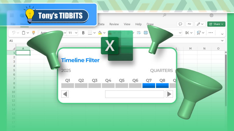 How to Create a Timeline Filter in ExcelApr 03, 2025 am 03:51 AM
In Excel, using the timeline filter can display data by time period more efficiently, which is more convenient than using the filter button. The Timeline is a dynamic filtering option that allows you to quickly display data for a single date, month, quarter, or year. Step 1: Convert data to pivot table First, convert the original Excel data into a pivot table. Select any cell in the data table (formatted or not) and click PivotTable on the Insert tab of the ribbon. Related: How to Create Pivot Tables in Microsoft Excel Don't be intimidated by the pivot table! We will teach you basic skills that you can master in minutes. Related Articles In the dialog box, make sure the entire data range is selected (
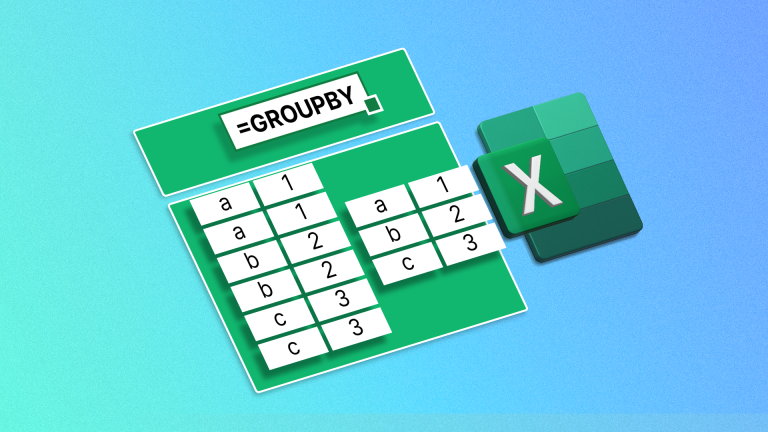 How to Use the GROUPBY Function in ExcelApr 02, 2025 am 03:51 AM
Excel's GROUPBY function: Powerful data grouping and aggregation tools Excel's GROUPBY function allows you to group and aggregate data based on specific fields in a data table. It also provides parameters that allow you to sort and filter the data so that you can customize the output to your specific needs. GROUPBY function syntax The GROUPBY function contains eight parameters: =GROUPBY(a,b,c,d,e,f,g,h) Parameters a to c are required: a (row field): A range (one column or multiple columns) containing the value or category to which the data is grouped. b (value): The range of values containing aggregated data (one column or multiple columns).
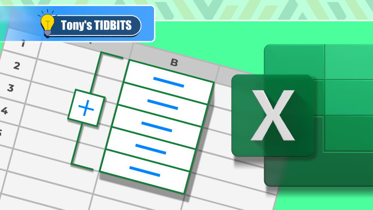 Don't Hide and Unhide Columns in Excel—Use Groups InsteadApr 01, 2025 am 12:38 AM
Excel efficient grouping: say goodbye to hidden columns and embrace flexible data management! While hidden columns can temporarily remove unnecessary data, grouping columns are often a better choice when dealing with large data sets or pursuing flexibility. This article will explain in detail the advantages and operation methods of Excel column grouping to help you improve data management efficiency. Why is grouping better than hiding? Hiding columns (right-click on the column title and select "Hide") can easily lead to data forgetting, even the column title prompt is not reliable because the title itself can be deleted. In contrast, grouped columns are faster and more convenient to expand and fold, which not only improves work efficiency, but also enhances user experience, especially when multi-person collaboration. Additionally, grouping columns allow creation of subgroups, which cannot be achieved by hidden columns. This is the number
 How to Completely Hide an Excel WorksheetMar 31, 2025 pm 01:40 PM
Excel worksheets have three levels of visibility: visible, hidden, and very hidden. Setting the worksheet to "very hidden" reduces the likelihood that others can access them. To set the worksheet to "very hidden", set its visibility to "xlsSheetVeryHidden" in the VBA window. Excel worksheets have three levels of visibility: visible, hidden, and very hidden. Many people know how to hide and unhide the worksheet by right-clicking on the tab area at the bottom of the workbook, but this is just a medium way to remove the Excel worksheet from the view. Whether you want to organize the workbook tabs, set up dedicated worksheets for drop-down list options and other controls, keeping only the most important worksheets visible, and
 Use the PERCENTOF Function to Simplify Percentage Calculations in ExcelMar 27, 2025 am 03:03 AM
Excel's PERCENTOF function: Easily calculate the proportion of data subsets Excel's PERCENTOF function can quickly calculate the proportion of data subsets in the entire data set, avoiding the hassle of creating complex formulas. PERCENTOF function syntax The PERCENTOF function has two parameters: =PERCENTOF(a,b) in: a (required) is a subset of data that forms part of the entire data set; b (required) is the entire dataset. In other words, the PERCENTOF function calculates the percentage of the subset a to the total dataset b. Calculate the proportion of individual values using PERCENTOF The easiest way to use the PERCENTOF function is to calculate the single


Hot AI Tools

Undresser.AI Undress
AI-powered app for creating realistic nude photos

AI Clothes Remover
Online AI tool for removing clothes from photos.

Undress AI Tool
Undress images for free

Clothoff.io
AI clothes remover

AI Hentai Generator
Generate AI Hentai for free.

Hot Article
Hot Tools

MantisBT
Mantis is an easy-to-deploy web-based defect tracking tool designed to aid in product defect tracking. It requires PHP, MySQL and a web server. Check out our demo and hosting services.

ZendStudio 13.5.1 Mac
Powerful PHP integrated development environment

SublimeText3 Chinese version
Chinese version, very easy to use

PhpStorm Mac version
The latest (2018.2.1) professional PHP integrated development tool

SecLists
SecLists is the ultimate security tester's companion. It is a collection of various types of lists that are frequently used during security assessments, all in one place. SecLists helps make security testing more efficient and productive by conveniently providing all the lists a security tester might need. List types include usernames, passwords, URLs, fuzzing payloads, sensitive data patterns, web shells, and more. The tester can simply pull this repository onto a new test machine and he will have access to every type of list he needs.

