


The article shows how to add colors to your data validation lists to make them more visually appealing and user-friendly.
You don't have to be an expert to make a drop-down menu in Excel or Google Sheets. But let's be honest - staring at a long list of values can be pretty boring. If you're looking to add some excitement to your spreadsheets, why not try highlighting a drop-down list with color? Whether you're organizing a list of products, categorizing expenses, or tracking sales data, a colored dropdown will make your data easier to read and understand. In this article, we'll show you how to do just that.

How to create Excel colored drop down list
If you use Excel for data entry, you've likely used the Data Validation feature to create drop-down lists. But did you know that you can also add colors to these lists? This section will guide you through the steps to colorize your drop-down list for a more eye-catching look.
Step 1. Create drop-down list
To add color to your Excel picklist, you first need to create the list itself. If you're unfamiliar with this process, refer to our separate article on creating a drop-down list that describes all possible methods in detail.
For this example, let's assume you have the source list of items in A3:A10 and you've created a drop-down menu with those items. To do that, simply select the range of cells where you want the dropdown to appear (D3:D12 in our case) and click the Data Validation button on the Data tab. In the Data Validation dialog box that appears, choose List from the Allow drop-down menu and, in the Source field, enter the reference to the range of cells containing your items.

Once you've created your drop-down list, you can move on to adding colors.
Step 2. Add colors to drop-down menu
To highlight your picklist with some color, we will be using Excel conditional formatting. The steps are:
- Select the cell(s) with your drop-down menu.
- On the Home tab, in the Styles group, click Conditional Formatting > New Rule… .
- In the New Formatting Rule dialog window, choose the Format only cells that contain option.
- Choose Specific Text from the first drop-down box and containing from the second drop-down box. In the third box, enter the reference to the cell containing the value that you want to format with a certain color like shown in the screenshot below. Alternatively, you can type the value enclosed in double quotes directly in the box, e.g. "Blue".

- Click the Format button.
- In the Format Cells dialog box, switch to the Fill tab, choose the color you like for that particular item, and click OK.
- Back in the New Formatting Rule dialog window, review the settings, and if everything looks good, click OK to save the changes.


Step 3. Test your colored drop-down list
To test your colored drop down menu, click on the arrow next to the cell. You should see the list of items you entered, with the first item highlighted in the chosen color:

Repeat the above steps for other selections and you will get a cohesive color scheme that makes it easy to visually distinguish between different selections.

Tips:
- If you've chosen dark fill colors for your drop-down list, selecting the white font color will make your options more readable. Similarly, if you've chosen light fill colors, using a dark font color will provide better contrast and readability.
- Don't be afraid to experiment with different color combinations to find the one that works best for your data!
- In Excel 365, you can use the brand new IMAGE function to create dropdown with pictures.
How to make Google Sheets drop down list with color
Google Sheets has become a go-to tool for many people. Like its Microsoft Excel counterpart, it offers the ability to create drop-down menus for easier data entry. With the latest version of Google spreadsheets, you no longer need to rely on conditional formatting tricks. Now, you can add colors to your data validation lists directly as you create them!
To create a colored drop-down list in Google Sheets, follow these steps:
- Select one or more cells where we want the dropdown list to appear.
- From the top toolbar, select Data and click Data validation.
- On the Data Validation rules pane, click Add rule.
- In the Criteria drop down menu, pick either the Dropdown or Dropdown from a range option.
- If you choose Dropdown, type your values in the Option 1 and Option 2 boxes, clicking the Add another item button as needed.
If you choose Dropdown from a range, type the range reference in the text field or use the Select Data Range button to pick the range. Either way, be sure to use absolute references with the $ sign to lock cell addresses such as e.g. =$D$4:$D$8.
- Once you've entered your options, it's time to add some color! Simply select the color you want for each item. If you need more tints than shown in the predefined palette, click Customize, and then choose a custom color.
- When you're finished, click the Done button.


There you have it - a colored drop-down menu that not only looks great, but also helps you organize and analyze your data more effectively.

How to create color-coded drop down list
In the first part of this tutorial, you learned how to create dropdown with colored text values. But what if you want to create a color-coded dropdown where only colors are visible, without any text values? This section will show you how to achieve that outcome. By selecting the same color for both the fill and font, you can create a monochromatic effect that is ideal for organizing data in a clear and concise way. Let's dive in and learn how to create a color coded dropdown list with hidden text values.
Color coded dropdown list in Excel
To make a color-coded dropdown in Excel worksheets, you set up conditional formatting rule as described in Adding colors to drop-down menu. When choosing the format, switch between the Fill and Font tabs and pick the same color on both.
Choosing the fill color:

Choosing the font color:

As a result, you will have a color-coded drop down list where each option is represented by a colored cell. This visual representation can be especially useful for data sets with a large number of categories or where color is a significant factor.

Color coded dropdown list in Google Sheets
To color code drop down list in Google Sheets, follow these steps. After adding background colors (Step 6), do the following:
- Click on the color you've added to a certain item, and then click Customize.
- On the Background tab, copy the Hex color code:
- On the Text tab, paste the copied hex code:


That's it! After following the steps outlined above, you'll have a color-coded dropdown menu effectively hiding the text values and leaving only the color swatches visible.

Note. Please remember that the purpose of visual communication is to enhance understanding, and different situations may require different visual cues to achieve that goal. Color codes are useful for representing data where the color is the primary indicator of meaning. However, if you need to provide additional context for each item, using different fill and font colors can be a more effective way to communicate this information visually.
In conclusion, adding color to drop-down lists in Excel and Google Sheets is a great way to enhance the visual appeal of your spreadsheets while also making them more functional and comprehensible. So go ahead and try it out, and see how color can transform your spreadsheets today!
Practice workbook for download
Excel color drop down list (.xlsx file) Google Sheets drop down list with color (online sheet)
以上がExcelとGoogleシートで色付きのドロップダウンリストを作成する方法の詳細内容です。詳細については、PHP 中国語 Web サイトの他の関連記事を参照してください。

 Excelの式の中央値 - 実用的な例Apr 11, 2025 pm 12:08 PM
このチュートリアルでは、中央値関数を使用してExcelの数値データの中央値を計算する方法について説明します。 中央傾向の重要な尺度である中央値は、データセットの中央値を識別し、中央の傾向のより堅牢な表現を提供します
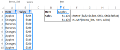
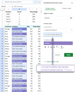 式の例を備えたGoogleスプレッドシートcountif機能Apr 11, 2025 pm 12:03 PM
マスターグーグルシートcountif:包括的なガイド このガイドでは、Googleシートの多用途のCountif機能を調査し、単純なセルカウントを超えてそのアプリケーションを実証しています。 正確な一致や部分的な一致から漢までのさまざまなシナリオをカバーします
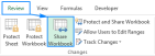 Excel共有ワークブック:複数のユーザーのExcelファイルを共有する方法Apr 11, 2025 am 11:58 AM
このチュートリアルは、さまざまな方法、アクセス制御、競合解決をカバーするExcelワークブックを共有するための包括的なガイドを提供します。 Modern Excelバージョン(2010、2013、2016、およびその後)共同編集を簡素化し、mの必要性を排除します
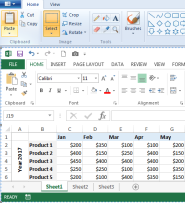 Excelをjpgに変換する方法 - .xlsまたは.xlsxを画像ファイルとして保存しますApr 11, 2025 am 11:31 AM
このチュートリアルでは、.xlsファイルを.jpg画像に変換するためのさまざまな方法を調査し、ビルトインWindowsツールと無料のオンラインコンバーターの両方を網羅しています。 プレゼンテーションを作成したり、スプレッドシートデータを安全に共有したり、ドキュメントを設計したりする必要がありますか?ヨーヨーを変換します
 名前と名前付き範囲:フォーミュラで定義および使用する方法Apr 11, 2025 am 11:13 AM
このチュートリアルは、Excel名の機能を明確にし、セル、範囲、定数、または式の名前を定義する方法を示します。 また、定義された名前の編集、フィルタリング、削除もカバーしています。 Excelの名前は、信じられないほど便利ですが、しばしばOverloです
 標準偏差Excel:関数と式の例Apr 11, 2025 am 11:01 AM
このチュートリアルは、標準偏差と平均の標準誤差の区別を明確にし、標準偏差計算のための最適なExcel関数を導きます。 記述統計では、平均および標準偏差は内在的です
 Excelの平方根:SQRT関数およびその他の方法Apr 11, 2025 am 10:34 AM
このExcelチュートリアルでは、正方形の根とNth Rootsを計算する方法を示しています。 平方根を見つけることは一般的な数学的操作であり、Excelはいくつかの方法を提供します。 Excelの正方形の根を計算する方法: SQRT関数を使用します
 Googleシートの基本:Googleスプレッドシートでの作業方法を学ぶApr 11, 2025 am 10:23 AM
Googleシートのパワーのロックを解除:初心者向けガイド このチュートリアルでは、MS Excelに代わる強力で多目的な代替品であるGoogleシートの基礎を紹介します。 スプレッドシートを簡単に管理し、重要な機能を活用し、コラボレーションする方法を学ぶ


ホットAIツール

Undresser.AI Undress
リアルなヌード写真を作成する AI 搭載アプリ

AI Clothes Remover
写真から衣服を削除するオンライン AI ツール。

Undress AI Tool
脱衣画像を無料で

Clothoff.io
AI衣類リムーバー

Video Face Swap
完全無料の AI 顔交換ツールを使用して、あらゆるビデオの顔を簡単に交換できます。

人気の記事
ホットツール

ZendStudio 13.5.1 Mac
強力な PHP 統合開発環境

WebStorm Mac版
便利なJavaScript開発ツール

SAP NetWeaver Server Adapter for Eclipse
Eclipse を SAP NetWeaver アプリケーション サーバーと統合します。

SublimeText3 英語版
推奨: Win バージョン、コードプロンプトをサポート!

MinGW - Minimalist GNU for Windows
このプロジェクトは osdn.net/projects/mingw に移行中です。引き続きそこでフォローしていただけます。 MinGW: GNU Compiler Collection (GCC) のネイティブ Windows ポートであり、ネイティブ Windows アプリケーションを構築するための自由に配布可能なインポート ライブラリとヘッダー ファイルであり、C99 機能をサポートする MSVC ランタイムの拡張機能が含まれています。すべての MinGW ソフトウェアは 64 ビット Windows プラットフォームで実行できます。

