


How to use Excel to perform sum operations
Step 1: Select the cells to be summed
- Click and drag mouse to select the range of cells to be summed.
Step 2: Click the Sum button
- On the Home tab, in the Editing group, click Sum button, which looks like a blue triangle with the Greek letter Σ on it.
Step 3: Select the summation function
- In the pop-up "AutoSum" drop-down menu, select the required summation function . The most commonly used function is Sum, which adds the values in all selected cells.
Step 4: Confirm Sum
- Make sure you have selected the correct range of cells and summation function.
- Click the "OK" button and Excel will insert the summation result below the selected cell.
Other sum functions
In addition to the basic "Sum" function, Excel also provides other sum functions, such as:
- SUMIF(): Sum cells if certain conditions are met.
- SUMIFS(): Sum the cells if multiple conditions are met.
- SUMPRODUCT(): Multiply and sum two or more arrays.
Tip
- Make sure the cells you want to sum are selected correctly.
- Use absolute references ($ signs) to ensure that the summation formula does not change when copied or moved.
- If the summation result is incorrect, check the formula and make sure there are no errors in the formula.
The above is the detailed content of How to operate sum in excel. For more information, please follow other related articles on the PHP Chinese website!

 Excel CONCATENATE function to combine strings, cells, columnsApr 30, 2025 am 10:23 AM
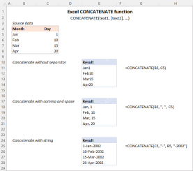
This article explores various methods for combining text strings, numbers, and dates in Excel using the CONCATENATE function and the "&" operator. We'll cover formulas for joining individual cells, columns, and ranges, offering solutio
 Merge and combine cells in Excel without losing dataApr 30, 2025 am 09:43 AM
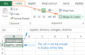
This tutorial explores various methods for efficiently merging cells in Excel, focusing on techniques to retain data when combining cells in Excel 365, 2021, 2019, 2016, 2013, 2010, and earlier versions. Often, Excel users need to consolidate two or
 Excel: Compare two columns for matches and differencesApr 30, 2025 am 09:22 AM
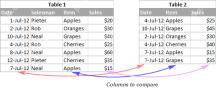
This tutorial explores various methods for comparing two or more columns in Excel to identify matches and differences. We'll cover row-by-row comparisons, comparing multiple columns for row matches, finding matches and differences across lists, high
 Rounding in Excel: ROUND, ROUNDUP, ROUNDDOWN, FLOOR, CEILING functionsApr 30, 2025 am 09:18 AM
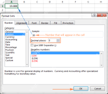
This tutorial explores Excel's rounding functions: ROUND, ROUNDUP, ROUNDDOWN, FLOOR, CEILING, MROUND, and others. It demonstrates how to round decimal numbers to integers or a specific number of decimal places, extract fractional parts, round to the
 Consolidate in Excel: Merge multiple sheets into oneApr 29, 2025 am 10:04 AM
This tutorial explores various methods for combining Excel sheets, catering to different needs: consolidating data, merging sheets via data copying, or merging spreadsheets based on key columns. Many Excel users face the challenge of merging multipl
 Calculate moving average in Excel: formulas and chartsApr 29, 2025 am 09:47 AM
This tutorial shows you how to quickly calculate simple moving averages in Excel, using functions to determine moving averages over the last N days, weeks, months, or years, and how to add a moving average trendline to your charts. Previous articles
 How to calculate average in Excel: formula examplesApr 29, 2025 am 09:38 AM
This tutorial demonstrates various methods for calculating averages in Excel, including formula-based and formula-free approaches, with options for rounding results. Microsoft Excel offers several functions for averaging numerical data, and this gui
 How to calculate weighted average in Excel (SUM and SUMPRODUCT formulas)Apr 29, 2025 am 09:32 AM
This tutorial shows you two simple ways to calculate weighted averages in Excel: using the SUM or SUMPRODUCT function. Previous articles covered basic Excel averaging functions. But what if some values are more important than others, impacting the f


Hot AI Tools

Undresser.AI Undress
AI-powered app for creating realistic nude photos

AI Clothes Remover
Online AI tool for removing clothes from photos.

Undress AI Tool
Undress images for free

Clothoff.io
AI clothes remover

Video Face Swap
Swap faces in any video effortlessly with our completely free AI face swap tool!

Hot Article
Hot Tools

SublimeText3 Chinese version
Chinese version, very easy to use

SAP NetWeaver Server Adapter for Eclipse
Integrate Eclipse with SAP NetWeaver application server.

SublimeText3 English version
Recommended: Win version, supports code prompts!

mPDF
mPDF is a PHP library that can generate PDF files from UTF-8 encoded HTML. The original author, Ian Back, wrote mPDF to output PDF files "on the fly" from his website and handle different languages. It is slower than original scripts like HTML2FPDF and produces larger files when using Unicode fonts, but supports CSS styles etc. and has a lot of enhancements. Supports almost all languages, including RTL (Arabic and Hebrew) and CJK (Chinese, Japanese and Korean). Supports nested block-level elements (such as P, DIV),

SecLists
SecLists is the ultimate security tester's companion. It is a collection of various types of lists that are frequently used during security assessments, all in one place. SecLists helps make security testing more efficient and productive by conveniently providing all the lists a security tester might need. List types include usernames, passwords, URLs, fuzzing payloads, sensitive data patterns, web shells, and more. The tester can simply pull this repository onto a new test machine and he will have access to every type of list he needs.

