
 Software TutorialOffice SoftwareHow to create an employee training tracker using Excel spreadsheets
1. Open EXCEL2013 - click on the category: Education - click on Employee Training Tracker.

2. After clicking on the employee training tracker, click: Create in the pop-up dialog box. At this time, the employee training tracker template will be downloaded and opened online.

3. The leader enters the name, department and position of the relevant training personnel in the personal information form of the personnel to be trained.

4. When training employees, write down the relevant training courses and training time - click on the course schedule, and then fill in the relevant requirements.

5. Click on the training log form - first fill in the training date, name, course, instructor, participation and passing status, etc. Most of them are optional.

6. Finally, check the training status of each employee: click on the training log - click on the employee name above to automatically filter out personal training information. You can also click on a certain course or the training status of a certain instructor to participate in the training.

The above is the detailed content of How to create an employee training tracker using Excel spreadsheets. For more information, please follow other related articles on the PHP Chinese website!

 How to Use AI Function in Google SheetsMay 03, 2025 am 06:01 AM
Google Sheets' AI Function: A Powerful New Tool for Data Analysis Google Sheets now boasts a built-in AI function, powered by Gemini, eliminating the need for add-ons to leverage the power of language models directly within your spreadsheets. This f
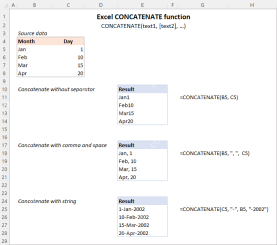 Excel CONCATENATE function to combine strings, cells, columnsApr 30, 2025 am 10:23 AM
This article explores various methods for combining text strings, numbers, and dates in Excel using the CONCATENATE function and the "&" operator. We'll cover formulas for joining individual cells, columns, and ranges, offering solutio
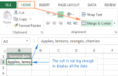 Merge and combine cells in Excel without losing dataApr 30, 2025 am 09:43 AM
This tutorial explores various methods for efficiently merging cells in Excel, focusing on techniques to retain data when combining cells in Excel 365, 2021, 2019, 2016, 2013, 2010, and earlier versions. Often, Excel users need to consolidate two or
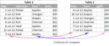 Excel: Compare two columns for matches and differencesApr 30, 2025 am 09:22 AM
This tutorial explores various methods for comparing two or more columns in Excel to identify matches and differences. We'll cover row-by-row comparisons, comparing multiple columns for row matches, finding matches and differences across lists, high
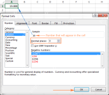 Rounding in Excel: ROUND, ROUNDUP, ROUNDDOWN, FLOOR, CEILING functionsApr 30, 2025 am 09:18 AM
This tutorial explores Excel's rounding functions: ROUND, ROUNDUP, ROUNDDOWN, FLOOR, CEILING, MROUND, and others. It demonstrates how to round decimal numbers to integers or a specific number of decimal places, extract fractional parts, round to the
 Consolidate in Excel: Merge multiple sheets into oneApr 29, 2025 am 10:04 AM
This tutorial explores various methods for combining Excel sheets, catering to different needs: consolidating data, merging sheets via data copying, or merging spreadsheets based on key columns. Many Excel users face the challenge of merging multipl
 Calculate moving average in Excel: formulas and chartsApr 29, 2025 am 09:47 AM
This tutorial shows you how to quickly calculate simple moving averages in Excel, using functions to determine moving averages over the last N days, weeks, months, or years, and how to add a moving average trendline to your charts. Previous articles
 How to calculate average in Excel: formula examplesApr 29, 2025 am 09:38 AM
This tutorial demonstrates various methods for calculating averages in Excel, including formula-based and formula-free approaches, with options for rounding results. Microsoft Excel offers several functions for averaging numerical data, and this gui


Hot AI Tools

Undresser.AI Undress
AI-powered app for creating realistic nude photos

AI Clothes Remover
Online AI tool for removing clothes from photos.

Undress AI Tool
Undress images for free

Clothoff.io
AI clothes remover

Video Face Swap
Swap faces in any video effortlessly with our completely free AI face swap tool!

Hot Article
Hot Tools

Dreamweaver CS6
Visual web development tools

PhpStorm Mac version
The latest (2018.2.1) professional PHP integrated development tool

WebStorm Mac version
Useful JavaScript development tools

Notepad++7.3.1
Easy-to-use and free code editor

Atom editor mac version download
The most popular open source editor

