


In Excel, subscripts usually refer to the coordinates of cells, such as A1, B2, etc. To type subscripts in Excel, you can use the following two methods. First, you can use special characters, such as subscript numbers in the Unicode character set. Secondly, the subscript effect can be achieved by inserting equations. For specific operations, please refer to the Excel help document, which details how to type subscripts in Excel. Hope the above method can help you!
1. Superscript method:
1. First, enter a3 (3 is superscript) in Excel.

#2. Select the number "3", right-click and select "Format Cells".

3. Click "Superscript" and then "OK".

4. Look, the effect is like this.

2. Subscript method:
1. Similar to the superscript setting method, enter "ln310" in the cell (3 is the subscript) , select the number "3", right-click and select "Format Cells".

#2. Check "Subscript" and click "OK".


3. Superscript and subscript methods without letters:
1. If the input content does not contain letters , for example, enter "33" (the second 3 is a superscript)". According to the above method, there is no way to set the superscript and subscript.
First, you must select the entire cell, right-click and set the cell format to "Text".

#2. Then select the second "3", right-click and set the cell format to "Superscript". Subscripts can also be set in the same way.


3. Finally, what we need to note is that we must set the cell format to text format before we can set the superscript and subscript, otherwise If so, the superscript and subscript may disappear after the settings are completed.
The above is the detailed content of How to type subscript in excel. For more information, please follow other related articles on the PHP Chinese website!

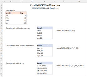 Excel CONCATENATE function to combine strings, cells, columnsApr 30, 2025 am 10:23 AM
This article explores various methods for combining text strings, numbers, and dates in Excel using the CONCATENATE function and the "&" operator. We'll cover formulas for joining individual cells, columns, and ranges, offering solutio
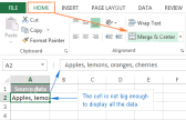 Merge and combine cells in Excel without losing dataApr 30, 2025 am 09:43 AM
This tutorial explores various methods for efficiently merging cells in Excel, focusing on techniques to retain data when combining cells in Excel 365, 2021, 2019, 2016, 2013, 2010, and earlier versions. Often, Excel users need to consolidate two or
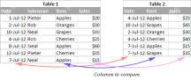 Excel: Compare two columns for matches and differencesApr 30, 2025 am 09:22 AM
This tutorial explores various methods for comparing two or more columns in Excel to identify matches and differences. We'll cover row-by-row comparisons, comparing multiple columns for row matches, finding matches and differences across lists, high
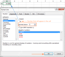 Rounding in Excel: ROUND, ROUNDUP, ROUNDDOWN, FLOOR, CEILING functionsApr 30, 2025 am 09:18 AM
This tutorial explores Excel's rounding functions: ROUND, ROUNDUP, ROUNDDOWN, FLOOR, CEILING, MROUND, and others. It demonstrates how to round decimal numbers to integers or a specific number of decimal places, extract fractional parts, round to the
 Consolidate in Excel: Merge multiple sheets into oneApr 29, 2025 am 10:04 AM
This tutorial explores various methods for combining Excel sheets, catering to different needs: consolidating data, merging sheets via data copying, or merging spreadsheets based on key columns. Many Excel users face the challenge of merging multipl
 Calculate moving average in Excel: formulas and chartsApr 29, 2025 am 09:47 AM
This tutorial shows you how to quickly calculate simple moving averages in Excel, using functions to determine moving averages over the last N days, weeks, months, or years, and how to add a moving average trendline to your charts. Previous articles
 How to calculate average in Excel: formula examplesApr 29, 2025 am 09:38 AM
This tutorial demonstrates various methods for calculating averages in Excel, including formula-based and formula-free approaches, with options for rounding results. Microsoft Excel offers several functions for averaging numerical data, and this gui
 How to calculate weighted average in Excel (SUM and SUMPRODUCT formulas)Apr 29, 2025 am 09:32 AM
This tutorial shows you two simple ways to calculate weighted averages in Excel: using the SUM or SUMPRODUCT function. Previous articles covered basic Excel averaging functions. But what if some values are more important than others, impacting the f


Hot AI Tools

Undresser.AI Undress
AI-powered app for creating realistic nude photos

AI Clothes Remover
Online AI tool for removing clothes from photos.

Undress AI Tool
Undress images for free

Clothoff.io
AI clothes remover

Video Face Swap
Swap faces in any video effortlessly with our completely free AI face swap tool!

Hot Article
Hot Tools

SAP NetWeaver Server Adapter for Eclipse
Integrate Eclipse with SAP NetWeaver application server.

VSCode Windows 64-bit Download
A free and powerful IDE editor launched by Microsoft

SublimeText3 Linux new version
SublimeText3 Linux latest version

mPDF
mPDF is a PHP library that can generate PDF files from UTF-8 encoded HTML. The original author, Ian Back, wrote mPDF to output PDF files "on the fly" from his website and handle different languages. It is slower than original scripts like HTML2FPDF and produces larger files when using Unicode fonts, but supports CSS styles etc. and has a lot of enhancements. Supports almost all languages, including RTL (Arabic and Hebrew) and CJK (Chinese, Japanese and Korean). Supports nested block-level elements (such as P, DIV),

Dreamweaver CS6
Visual web development tools

