

How to use vlookup function to match across tables

The vlookup function is one of the most commonly used functions in Excel. It can help us find a specified value in a table and return the corresponding value in another table that matches the value. In this article, we will explore the use of the vlookup function, especially when performing cross-table matching.
First, let us learn the basic syntax of the vlookup function. In Excel, the syntax of the vlookup function is as follows:
=vlookup(lookup_value, table_array, col_index, range_lookup)
where:
- lookup_value: to be in the table The value to look for.
- table_array: The table area to be matched, including the value to be searched and the corresponding matching value.
- col_index: The number of columns where the corresponding value is to be returned. If the first column of table_array is a matching value, col_index is 1, the second column is 2, and so on.
- range_lookup: A Boolean value used to determine whether to perform an exact match. If TRUE, an approximate match is made; if FALSE, an exact match is made.
Next, we will use an example to demonstrate the use of the vlookup function. Suppose we have two tables, one is the product list table and the other is the price table. The product list table contains the product name and the corresponding product number, while the price table contains the product number and the corresponding price.
In this example, we need to find the corresponding product price in the price table based on the product number in the product list table.
First, we need to add a column to the product list table to store the product price. We can insert a column to the right of the third column to store prices. Then, enter the following formula in the first cell:
=vlookup(B2, price table!A:B, 2, FALSE)
This formula means: In the price table Find the value in the first column that matches cell B2 in the second column, and return the matching value in the second column. Since we want an exact match, the range_lookup parameter is set to FALSE.
Next, we need to drag or copy this formula to all cells in the product list table to apply the formula to the entire column.
Once we complete these steps, the third column in the item list table will display the item price corresponding to the item number.
It should be noted that if the product number in the product list table cannot find the corresponding price in the price table, the vlookup function will return the error value #N/A. This indicates that the item number does not exist in the price table, or there may be some other error.
In addition, there are some details that need attention. First, the vlookup function only works when the first column of the search area is a key value. Therefore, before using the vlookup function, we should adjust the column order of the search area to ensure that the target column is in the first column. Secondly, if we find duplicate values in the search area, the vlookup function will return the first matching value encountered.
To summarize, by using the vlookup function, we can easily perform cross-table matching between different tables. Whether in business data analysis or daily work, the vlookup function is a very powerful and practical tool. Hope this article can help you better understand and apply the vlookup function.
The above is the detailed content of How to use vlookup function to match across tables. For more information, please follow other related articles on the PHP Chinese website!

 I Use Custom Number Formatting Instead of Conditional Formatting in ExcelMay 06, 2025 am 12:56 AM
Detailed explanation of custom number formats: Quickly create personalized number formats in Excel Excel provides a variety of data formatting tools, but sometimes built-in tools are not able to meet specific needs or are inefficient. At this point, custom digital formats can come in handy to quickly create digital formats that meet your needs. What is a custom number format and how it works? In Excel, each cell has its own number format, which you can view by selecting the cell and in the Number group on the Start tab of the ribbon. Related: Excel's 12 digital format options and their impact on data Adjust the number format of the cell to match its data type. You can click on the "Number Format" dialog launcher and then
 How to Use the CHOOSECOLS and CHOOSEROWS Functions in Excel to Extract DataMay 05, 2025 am 03:02 AM
Excel's CHOOSECOLS and CHOOSEROWS functions simplify extracting specific columns or rows from data, eliminating the need for nested formulas. Their dynamic nature ensures they adapt to dataset changes. CHOOSECOLS and CHOOSEROWS Syntax: These functio
 How to Use AI Function in Google SheetsMay 03, 2025 am 06:01 AM
Google Sheets' AI Function: A Powerful New Tool for Data Analysis Google Sheets now boasts a built-in AI function, powered by Gemini, eliminating the need for add-ons to leverage the power of language models directly within your spreadsheets. This f
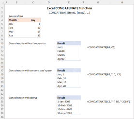 Excel CONCATENATE function to combine strings, cells, columnsApr 30, 2025 am 10:23 AM
This article explores various methods for combining text strings, numbers, and dates in Excel using the CONCATENATE function and the "&" operator. We'll cover formulas for joining individual cells, columns, and ranges, offering solutio
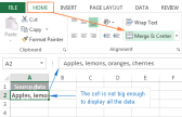 Merge and combine cells in Excel without losing dataApr 30, 2025 am 09:43 AM
This tutorial explores various methods for efficiently merging cells in Excel, focusing on techniques to retain data when combining cells in Excel 365, 2021, 2019, 2016, 2013, 2010, and earlier versions. Often, Excel users need to consolidate two or
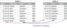 Excel: Compare two columns for matches and differencesApr 30, 2025 am 09:22 AM
This tutorial explores various methods for comparing two or more columns in Excel to identify matches and differences. We'll cover row-by-row comparisons, comparing multiple columns for row matches, finding matches and differences across lists, high
 Rounding in Excel: ROUND, ROUNDUP, ROUNDDOWN, FLOOR, CEILING functionsApr 30, 2025 am 09:18 AM
This tutorial explores Excel's rounding functions: ROUND, ROUNDUP, ROUNDDOWN, FLOOR, CEILING, MROUND, and others. It demonstrates how to round decimal numbers to integers or a specific number of decimal places, extract fractional parts, round to the
 Consolidate in Excel: Merge multiple sheets into oneApr 29, 2025 am 10:04 AM
This tutorial explores various methods for combining Excel sheets, catering to different needs: consolidating data, merging sheets via data copying, or merging spreadsheets based on key columns. Many Excel users face the challenge of merging multipl


Hot AI Tools

Undresser.AI Undress
AI-powered app for creating realistic nude photos

AI Clothes Remover
Online AI tool for removing clothes from photos.

Undress AI Tool
Undress images for free

Clothoff.io
AI clothes remover

Video Face Swap
Swap faces in any video effortlessly with our completely free AI face swap tool!

Hot Article
Hot Tools

Notepad++7.3.1
Easy-to-use and free code editor

mPDF
mPDF is a PHP library that can generate PDF files from UTF-8 encoded HTML. The original author, Ian Back, wrote mPDF to output PDF files "on the fly" from his website and handle different languages. It is slower than original scripts like HTML2FPDF and produces larger files when using Unicode fonts, but supports CSS styles etc. and has a lot of enhancements. Supports almost all languages, including RTL (Arabic and Hebrew) and CJK (Chinese, Japanese and Korean). Supports nested block-level elements (such as P, DIV),

Zend Studio 13.0.1
Powerful PHP integrated development environment

VSCode Windows 64-bit Download
A free and powerful IDE editor launched by Microsoft

DVWA
Damn Vulnerable Web App (DVWA) is a PHP/MySQL web application that is very vulnerable. Its main goals are to be an aid for security professionals to test their skills and tools in a legal environment, to help web developers better understand the process of securing web applications, and to help teachers/students teach/learn in a classroom environment Web application security. The goal of DVWA is to practice some of the most common web vulnerabilities through a simple and straightforward interface, with varying degrees of difficulty. Please note that this software

