


How to find specified data in large batches using Excel
1. Use VLOOKUP and MATCH functions together. Formula idea: The MATCH function searches for the name and address, that is, the column number; the vlookup function searches for the data.
The formula is: =VLOOKUP(b1,sheet1!a1:g300,MATCH(b2,sheet1!b1:G1),0), the specific data range is adjusted according to your table.
2. Usage of vlookup function.
The syntax format of the vlookup function:
=vlookup(lookup_value,table_array,col_index_num, range_lookup)
=vlookup (the value searched in the first column of the data table, the search range, the column in which the returned value is in the search range, fuzzy matching/exact matching)
FALSE(0) Omitted for exact match.
TRUE(1) is an approximate match.
3. Usage of MATCH function.
Syntax format of function:
=MATCH(lookup_value,lookuparray,match-type)
lookup_value: Indicates the specified content of the query;
lookuparray: indicates the specified area of the query;
match-type: Indicates the query specification method, represented by the number -1, 0 or 1
How to find the same data in two sets of data
1
Methods to move or copy tables:
Assuming that these two tables are not in the same excel, move them to the same table
2
Syntax of Vlookup function:
VLOOKUP(lookup_value,table_array,col_index_num,range_lookup)
lookup_value: The value to look for, a numeric value, a reference or a text string
table_array: area to be searched, data table area
col_index_num: Returns the column number of the data in the area, a positive integer
range_lookup: fuzzy matching, TRUE (or not filled in) /FALSE
3
Find two columns of identical data:
The formula used is =VLOOKUP(A2,Sheet2!A:B,1,0)
The meaning of the formula is to find the value equal to a2 in the first column of the A:B area of the sheet2 worksheet. After finding it, return the value of the same row in the first column of the area (i.e. column E). The last parameter 0 means exact search.
4
Find the data corresponding to the two columns:
The formula used is =VLOOKUP(A2,Sheet2!$A$2:B150,2,0)
The meaning of the formula is to find the value in column B that meets the conditions in the A2:B150 area of the sheet2 worksheet. After finding it, return the value of the same row in column 2 (i.e. column F) of the area. The last parameter 0 means exact search.
5
After completing the above four steps, the last step is relatively simple. Just pull the filling handle to fill the blank space below. The corresponding data will be displayed directly if it is found. If it is not found, #N/A will be displayed.
The above is the detailed content of Learn how to find specific data in batches using Excel. For more information, please follow other related articles on the PHP Chinese website!

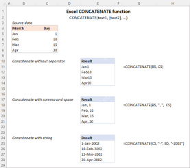 Excel CONCATENATE function to combine strings, cells, columnsApr 30, 2025 am 10:23 AM
This article explores various methods for combining text strings, numbers, and dates in Excel using the CONCATENATE function and the "&" operator. We'll cover formulas for joining individual cells, columns, and ranges, offering solutio
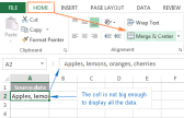 Merge and combine cells in Excel without losing dataApr 30, 2025 am 09:43 AM
This tutorial explores various methods for efficiently merging cells in Excel, focusing on techniques to retain data when combining cells in Excel 365, 2021, 2019, 2016, 2013, 2010, and earlier versions. Often, Excel users need to consolidate two or
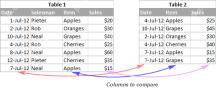 Excel: Compare two columns for matches and differencesApr 30, 2025 am 09:22 AM
This tutorial explores various methods for comparing two or more columns in Excel to identify matches and differences. We'll cover row-by-row comparisons, comparing multiple columns for row matches, finding matches and differences across lists, high
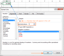 Rounding in Excel: ROUND, ROUNDUP, ROUNDDOWN, FLOOR, CEILING functionsApr 30, 2025 am 09:18 AM
This tutorial explores Excel's rounding functions: ROUND, ROUNDUP, ROUNDDOWN, FLOOR, CEILING, MROUND, and others. It demonstrates how to round decimal numbers to integers or a specific number of decimal places, extract fractional parts, round to the
 Consolidate in Excel: Merge multiple sheets into oneApr 29, 2025 am 10:04 AM
This tutorial explores various methods for combining Excel sheets, catering to different needs: consolidating data, merging sheets via data copying, or merging spreadsheets based on key columns. Many Excel users face the challenge of merging multipl
 Calculate moving average in Excel: formulas and chartsApr 29, 2025 am 09:47 AM
This tutorial shows you how to quickly calculate simple moving averages in Excel, using functions to determine moving averages over the last N days, weeks, months, or years, and how to add a moving average trendline to your charts. Previous articles
 How to calculate average in Excel: formula examplesApr 29, 2025 am 09:38 AM
This tutorial demonstrates various methods for calculating averages in Excel, including formula-based and formula-free approaches, with options for rounding results. Microsoft Excel offers several functions for averaging numerical data, and this gui
 How to calculate weighted average in Excel (SUM and SUMPRODUCT formulas)Apr 29, 2025 am 09:32 AM
This tutorial shows you two simple ways to calculate weighted averages in Excel: using the SUM or SUMPRODUCT function. Previous articles covered basic Excel averaging functions. But what if some values are more important than others, impacting the f


Hot AI Tools

Undresser.AI Undress
AI-powered app for creating realistic nude photos

AI Clothes Remover
Online AI tool for removing clothes from photos.

Undress AI Tool
Undress images for free

Clothoff.io
AI clothes remover

Video Face Swap
Swap faces in any video effortlessly with our completely free AI face swap tool!

Hot Article
Hot Tools

Dreamweaver Mac version
Visual web development tools

SublimeText3 English version
Recommended: Win version, supports code prompts!

SublimeText3 Mac version
God-level code editing software (SublimeText3)

VSCode Windows 64-bit Download
A free and powerful IDE editor launched by Microsoft

Zend Studio 13.0.1
Powerful PHP integrated development environment

