Summary of computational complexity of eight common machine learning algorithms

Computational complexity is a measure of the computing resources (time and space) consumed by a specific algorithm when running.

Computational complexity is divided into two categories:

1. Time complexity

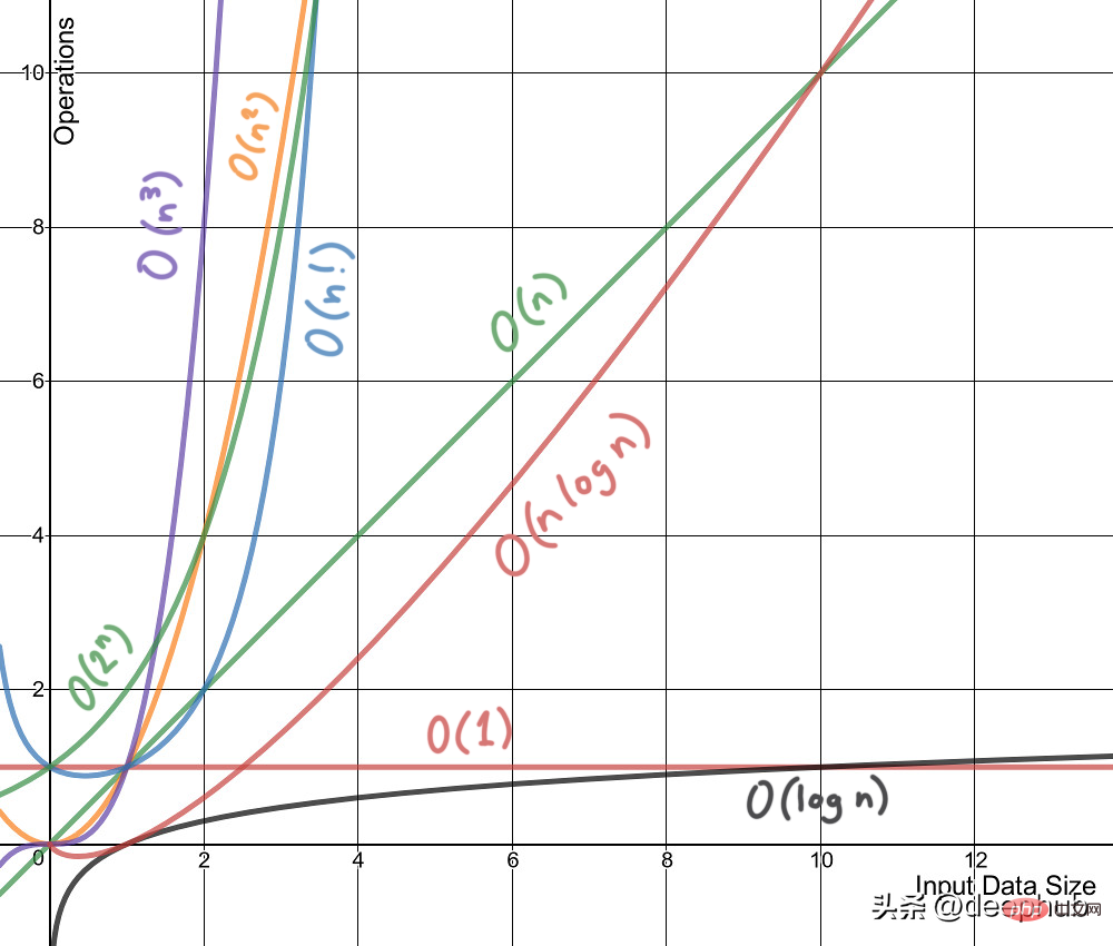
Time complexity is not a measure of an algorithm or a piece of code running under a certain machine or condition. time spent. Time complexity generally refers to time complexity, which is a function that qualitatively describes the running time of the algorithm and allows us to compare different algorithms without running them. For example, an algorithm with O(n) will always perform better than O(n²) because its growth rate is less than O(n²).

2. Space complexity

Just like time complexity is a function, so is space complexity. Conceptually it's the same as time complexity, just replace time with space. Wikipedia defines space complexity as:

The space complexity of an algorithm or computer program is the amount of storage space required to solve an instance of a computational problem as a function of the number of features as input.

Below we have compiled the computational complexity of some common machine learning algorithms.

1. Linear regression

• n=number of training samples, f = number of features
• Training time complexity: O(f²n f³)
• Prediction time complexity: O(f)
• Runtime space complexity: O(f)

2. Logistic regression:

• n = number of training samples, f = number of features
• Training time complexity: O(f*n)
• Prediction time complexity: O(f)
• Runtime space Complexity: O(f)

3. Support vector machine:

• n=number of training samples, f=number of features, s=number of support vectors
• Training time complexity: O(n²) to O(n³), training time complexity varies with different kernels.
• Predicted time complexity: O(f) to O(s*f): linear kernel is O(f), RBF and polynomial is O(s*f)
• Runtime space Complexity: O(s)

4. Naive Bayes:

• n=number of training samples, f=number of features, c=number of categories for classification
• Training time complexity: O(n*f*c)
• Prediction time complexity: O(c*f)
• Runtime space complexity: O(c *f)

5. Decision tree:

• n=number of training samples, f=number of features, d=depth of tree, p=number of nodes
• Training time complexity: O(n*log(n)*f)
• Prediction time complexity: O(d)
• Runtime space complexity: O(p)

6. Random forest:

• n= number of training samples, f = number of features, k = number of trees, p = number of nodes in the tree, d = Depth of tree
• Training time complexity: O(n*log(n)*f*k)
• Prediction time complexity: O(d*k)
• Runtime space complexity: O(p*k)

7, K nearest neighbor:

n=number of training samples, f=number of features, k=number of nearest neighbors

Brute:

• Training time complexity: O(1)
• Prediction time complexity: O(n*f k*f)
• Runtime Space complexity: O(n*f)

kd-tree:

• Training time complexity: O(f*n*log(n))
• Prediction time complexity: O(k*log(n))
• Runtime space complexity: O(n*f)

8, K-means Clustering:

• n= number of training samples, f = number of features, k= number of clusters, i = number of iterations
• Training time complexity: O(n*f*k *i)
• Runtime space complexity: O(n*f k*f)

The above is the detailed content of Summary of computational complexity of eight common machine learning algorithms. For more information, please follow other related articles on the PHP Chinese website!