Use handcrafted features to improve model performance

By performing hand-crafted feature engineering on raw data, we can take model accuracy and performance to new levels, paving the way for more accurate predictions and smarter business decisions. Models can be optimized like never before. and improve business capabilities.

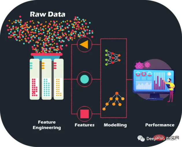
Raw data is like a jigsaw puzzle without a picture - but with feature engineering we can put the pieces together, although having large amounts of data is indeed a challenge in the quest to build machines A treasure trove of learning models for financial institutions, but it’s also important to acknowledge that not all data is informative. Moreover, the manual features are designed manually, and the reasons for each operation can be explained, which also brings interpretability.

Feature engineering is more than just selecting the best features. It also involves reducing noise and redundancy in the data to improve the generalization ability of the model. This is crucial because models need to perform well on unseen data to be truly useful.

Dataset Description

The dataset described in this article has been anonymized and masked to maintain the confidentiality of customer data. Features can be classified as follows:

D_* = 拖欠变量
S_* = 支出变量
P_* = 支付变量
B_* = 平衡变量
R_* = 风险变量

There are a total of 100 integer features and 100 floating point features representing the status of the customer in the past 12 months. This dataset contains information about customer reports ranging from 1 to 13. There may be a gap of 30 to 180 days between each of a customer's credit card statements (i.e., a customer's credit card statement may be missing). Each customer is represented by a customer ID. The sample data of the first 5 customers with customer_ID=0 is as follows:

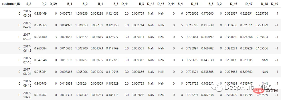
Among the 7 million customer_IDs, 98% of the labels are "0" (good customers, none Default), 2% are labeled "1" (Bad Customer, Default).

The data set is large, so we use cudf to speed up processing. If you do not have cudf installed, it is the same with pandas.

# LOAD LIBRARIES
 import pandas as pd, numpy as np # CPU libraries
 import cudf # GPU libraries
 import matplotlib.pyplot as plt, gc, os
 
 df = cudf.read_parquet('./data.parquet')

Feature generation methods

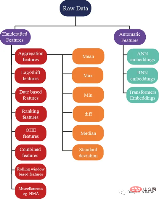
There are hundreds Several ideas can be used to generate features; but we also ensure that these features help improve the performance of the model. The following figure shows some basic methods used in feature engineering:

Aggregation Feature

Aggregation is the secret to understanding complex data. By calculating summary statistics for categorical grouping variables such as customer_ID (C_ID) or product category, or aggregations of numeric variables, we can discover invisible patterns and trends. With summary statistics like mean, maximum, minimum, standard deviation, and median, we can build more accurate predictive models and extract meaningful insights from customer data, transaction data, or any other numerical data.

These statistical attributes can be calculated for each customer

cat_features = ["B_1","B_2","D_1","D_2","D_10","P_21","D_126","D_3","D_42","R_66","R_68"]
 num_features = [col for col in all_cols if col not in cat_features] #all features accept cateforical features.
 test_num_agg = df.groupby("customer_ID")[num_features].agg(['mean', 'std', 'min', 'max', 'last','median']) #grouping by customerID
 test_num_agg.columns = ['_'.join(x) for x in test_num_agg.columns]

Mean: The average value of a numerical variable can give a general sense of the central tendency of the data. The average captures:

The average bank balance a customer has.

• Average customer spend.
• The average time between two credit statements (the time between credit payments).
• The average risk of borrowing money.

Standard Deviation (Std): A measure of the distribution of data around the mean, which can provide insight into the degree of variation in the data. High variability in balances indicates that customers are spending.

Minimum and maximum values ​​capture a client's wealth and also capture information about a client's spending and risk.

Median: When the data is highly skewed, using the mean is not a better idea, so the median can be used (the middle of the values ​​can be used.

The latest value may be The most important features because they contain information about the latest known credit statement issued to the customer, indicating the current status of the customer's account.

One-Hot Encoding

Use for categorical variables The above statistical properties are unwise because calculating minimum, maximum or standard deviation does not give us any useful information. So what should we do? Features can be calculated using features like count, and unique quantities, The latest value can also be obtained using

cat_features = ["B_1","B_2","D_1","D_2","D_10","P_21","D_126","D_3","D_42","R_66","R_68"]
 test_cat_agg = df.groupby("customer_ID")[cat_features].agg(['count', 'last', 'nunique'])
 test_cat_agg.columns = ['_'.join(x) for x in test_cat_agg.columns]

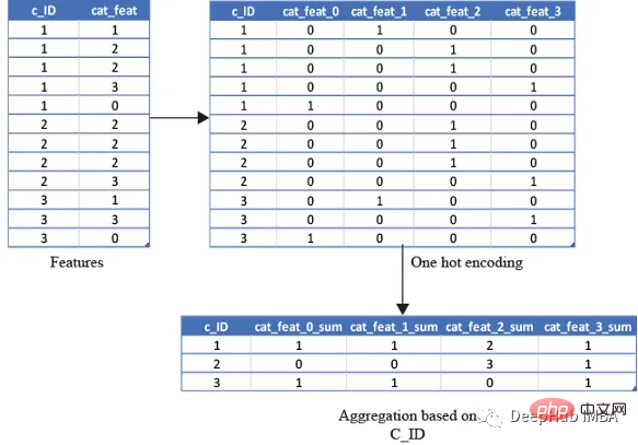
but this information does not capture whether the customer is categorized into a specific category or not. So we do this by one hot encoding the variables and then encoding the variables such as mean, sum and finally ) to achieve this by aggregating.

The average will capture the ratio of the total number of times a customer falls into that category/total number of bank statements. The sum will simply be the total number of times a customer falls into that category.

from cuml.preprocessing import OneHotEncoder
 df_categorical = df_last[cat_features].astype(object)
 ohe = OneHotEncoder(drop='first', sparse=False, dtype=np.float32, handle_unknown='ignore')
 ohe.fit(df_categorical)with open("ohe.pickle", 'wb') as f:
pickle.dump(ohe, f) #save the encoder so that it can be used for test data as well df_categorical = pd.DataFrame(ohe.transform(df_categorical).astype(np.float16),index=df_categorical.index).rename(columns=str)
 df_categorical['customer_ID']=df['customer_ID']
 df_categorical.groupby('customer_ID').agg(['mean', 'sum', 'last'])

基于排名的特征

在预测客户行为方面，基于排名的特征是非常重要的。通过根据收入或支出等特定属性对客户进行排名，我们可以深入了解他们的财务习惯并更好地管理风险。

使用 cudf 的 rank 函数，我们可以轻松计算这些特征并使用它们来为预测提供信息。例如，可以根据客户的消费模式、债务收入比或信用评分对客户进行排名。然后这些特征可用于预测违约或识别有可能拖欠付款的客户。

基于排名的特征还可用于识别高价值客户、目标营销工作和优化贷款优惠。例如，可以根据客户接受贷款提议的可能性对客户进行排名，然后将排名最高的客户作为目标。

df[feat+'_rank']=df[feat].rank(pct=True, method='min')

PCT用于是否做百分位排名。客户的排名也可以基于分类特征来计算。

df[feat+'_rank']=df.groupby([cat_feat]).rank(pct=True, method='min')

特征组合

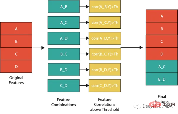
特征组合的一种流行方法是线性或非线性组合。这包括采用两个或多个现有特征，将它们组合在一起创建一个新的复合特征。然后使用这个复合特征来识别单独查看单个特征时可能不可见的模式、趋势和相关性。

例如，假设我们正在分析客户消费习惯的数据集。可以从个人特征开始，比如年龄、收入和地点。但是通过以线性或非线性的方式组合这些特性，可以创建新的复合特性，使我们能够更多地了解客户。可以结合收入和位置来创建一个复合特征，该特征告诉我们某一地区客户的平均支出。

但是并不是所有的特征组合都有用。关键是要确定哪些组合与试图解决的问题最相关，这需要对数据和问题领域有深刻的理解，并仔细分析创建的复合特征和试图预测的目标变量之间的相关性。

下图展示了一个组合特征并将信息用于模型的过程。作为筛选条件，这里只选择那些与目标相关性大于最大值 0.9 的特征。

features=[col for col in train.columns if col not in ['customer_ID',target]+cat_features]
 for feat1 in features:
for feat2 in features:
th=max(np.corr(feat1,Y)[0],np.corr(feat1,Y)[0]) #calculate threshold
feat3=df[feat1]-df[feat2] #difference feature
corr3=np.corr(feat3,Y)[0]
if(corr3>max(th,0.9)): #if correlation greater than max(th,0.9) we add it as feature
df[feat1+'_'+feat2]=feat3

基于时间/日期的特征

在数据分析方面，基于时间的特征非常重要。通过根据时间属性（例如月份或星期几）对数据进行分组，可以创建强大的特征。这些特征的范围可以从简单的平均值（如收入和支出）到更复杂的属性（如信用评分随时间的变化）。

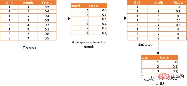
借助基于时间的特征，还可以识别在孤立地查看数据时可能看不到的模式和趋势。下图演示了如何使用基于时间的特征来创建有用的复合属性。

首先，计算一个月内的值的平均值（可以使用该月的某天或该月的某周等），将获得的DF与原始数据合并，并取各个特征之间的差。

features=[col for col in train.columns if col not in ['customer_ID',target]+cat_features]
 month_Agg=df.groupby([month])[features].agg('mean')#grouping based on month feature
 month_Agg.columns = ['_month_'.join(x) for x in month_Agg.columns]
 month_Agg.reset_index(inplace=True)
 df=df.groupby(month_Agg,notallow='month')
 for feat in features: #create composite features b taking difference
df[feat+'_'+feat+'_month_mean']=df[feat]-df[feat+'_month_mean']

还可以通过使用时间作为分组变量来创建基于排名的特征，如下所示

features=[col for col in train.columns if col not in ['customer_ID',target]+cat_features]
 month_Agg=df.groupby([month])[features].rank(pct=True) #grouping based on month feature
 month_Agg.columns = ['_month_'.join(x) for x in month_Agg.columns]
 month_Agg.reset_index(inplace=True)
 df=pd.concat([df,month_Agg],axis=1) #concat to original dataframe

滞后特征

滞后特征是有效预测金融数据的重要工具。这些特征包括计算时间序列中当前值与之前值之间的差值。通过将滞后特征纳入分析，可以更好地理解数据中的模式和趋势，并做出更准确的预测。

如果滞后特征显示客户连续几个月按时支付信用卡账单，可能会预测他们将来不太可能违约。相反，如果延迟特征显示客户一直延迟或错过付款，可能会预测他们更有可能违约。

# difference function calculate the lag difference for numerical features
 #between last value and shift last value.
 def difference(groups,num_features,shift):
data=(groups[num_features].nth(-1)-groups[num_features].nth(-1*shift)).rename(columns={f: f"{f}_diff{shift}" for f in num_features})
return data
 #calculate diff features for last -2nd last, last -3rd last, last- 4th last
 def get_difference(data,num_features):
print("diff features...")
groups=data.groupby('customer_ID')
df1=difference(groups,num_features,2).fillna(0)
df2=difference(groups,num_features,3).fillna(0)
df3=difference(groups,num_features,4).fillna(0)
df1=pd.concat([df1,df2,df3],axis=1)
df1.reset_index(inplace=True)
df1.sort_values(by='customer_ID')
del df2,df3
gc.collect()
return df1train_diff = get_difference(df, num_features)

基于滚动窗口的特性

这些特征只是取最后3(4,5，…x)值的平均值，这取决于数据，因为基于时间的最新值携带了关于客户最新状态的信息。

xth=3 #define the window size
 df["cumulative"]=df.groupby('customer_ID').sort_values(by=['time'],ascending=False).cumcount()
 last_info=df[df["cumulative"]<=xth]
 last_info = last_info.groupby("customer_ID")[num_features].agg(['mean', 'std', 'min', 'max', 'last','median']) #grouping by customerID
 last_info.columns = ['_'.join(x) for x in last_info.columns]

其他的特征提取方法

上面的方法已经创建了足够多的特征来构建一个很棒的模型。但是根据数据的性质，还可以创建更多的特征。例如：可以创建像null计数这样的特征，它可以计算客户当前的总null值，从而帮助捕获基于树的算法无法理解的特征分布。

def calc_nan(df,features):
print("calculating nan_info...")
df_nan = (df[features].mul(0) + 1).fillna(0) #marke non_null values as 1 and null as zero
df_nan['customer_ID'] = df['customer_ID']
nan_sum = df_nan.groupby("customer_ID").sum().sum(axis=1) #total unknown values for a customer
nan_last = df_nan.groupby("customer_ID").last().sum(axis=1)#how many last values that are not known
del df_nan
gc.collect()
return nan_sum,nan_last

这里可以不使用平均值，而是使用修正的平均值，如基于时间的加权平均值或 HMA(hull moving average)。

Summary

In this article we have presented some of the most common handcrafted feature strategies used to predict default risk in the real world. But there are always new and innovative ways to design features, and the method of manually setting features is time-consuming and laborious, so we will introduce how to use tools for automatic feature generation in a later article.

The above is the detailed content of Use handcrafted features to improve model performance. For more information, please follow other related articles on the PHP Chinese website!