Home >Technology peripherals >AI >Integrating time series models to improve forecast accuracy
Integrating time series models to improve forecast accuracy
- PHPzforward
- 2023-05-11 09:10:051128browse
Use Catboost to extract signals from RNN, ARIMA and Prophet models for prediction.
Integrating various weak learners can improve prediction accuracy, but if our model is already very powerful, ensemble learning can often be the icing on the cake. The popular machine learning library scikit-learn provides a StackingRegressor that can be used for time series tasks. But StackingRegressor has a limitation; it only accepts other scikit-learn model classes and APIs. So models like ARIMA that are not available in scikit-learn, or models from deep neural networks cannot be used. In this post I will show how to stack the predictions of the model that we can see.

We will use the following package:
pip install --upgrade scalecast
 conda install tensorflow
 conda install shap
 conda install -c conda-forge cmdstanpy
 pip install prophet
Dataset
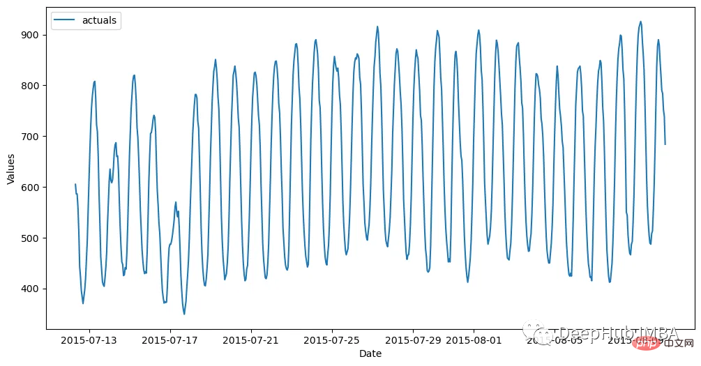
The data set is generated hourly and divided into a training set (700 observations) and a test set (48 observations). The following code reads the data and stores it in the Forecaster object:
import pandas as pd
 import numpy as np
 from scalecast.Forecaster import Forecaster
 from scalecast.util import metrics
 import matplotlib.pyplot as plt
 import seaborn as sns

 def read_data(idx = 'H1', cis = True, metrics = ['smape']):
 info = pd.read_csv(
 'M4-info.csv',
 index_col=0,
 parse_dates=['StartingDate'],
 dayfirst=True,
)
 train = pd.read_csv(
 f'Hourly-train.csv',
 index_col=0,
).loc[idx]
 test = pd.read_csv(
 f'Hourly-test.csv',
 index_col=0,
).loc[idx]
 y = train.values
 sd = info.loc[idx,'StartingDate']
 fcst_horizon = info.loc[idx,'Horizon']
 cd = pd.date_range(
 start = sd,
 freq = 'H',
 periods = len(y),
)
 f = Forecaster(
 y = y, # observed values
 current_dates = cd, # current dates
 future_dates = fcst_horizon, # forecast length
 test_length = fcst_horizon, # test-set length
 cis = cis, # whether to evaluate intervals for each model
 metrics = metrics, # what metrics to evaluate
)

 return f, test.values

 f, test_set = read_data()
 f # display the Forecaster object
The result is like this:

Model
Before we start building the model, we need to generate the simplest prediction from it. The naive method is to propagate forward the most recent 24 observations.
f.set_estimator('naive')
 f.manual_forecast(seasonal=True)
Then use ARIMA, LSTM and Prophet as benchmarks.
ARIMA
Autoregressive Integrated Moving Average is a popular and simple time series technique that uses the lag and error of a series to predict its future in a linear manner. Through EDA, we determined that this series is highly seasonal. So I finally chose to apply the seasonal ARIMA model of order (5,1,4) x(1,1,1,24).
f.set_estimator('arima')
 f.manual_forecast(
order = (5,1,4),
seasonal_order = (1,1,1,24),
call_me = 'manual_arima',
 )
LSTM
If ARIMA is a relatively simple time series model, then LSTM is one of the more advanced methods. It is a deep learning technique with many parameters, including a mechanism for discovering long-term and short-term patterns in sequential data, which theoretically makes it ideal for time series. Here is using tensorflow to build this model
f.set_estimator('rnn')
 f.manual_forecast(
 lags = 48,
 layers_struct=[
('LSTM',{'units':100,'activation':'tanh'}),
('LSTM',{'units':100,'activation':'tanh'}),
('LSTM',{'units':100,'activation':'tanh'}),
],
 optimizer = 'Adam',
 epochs = 15,
 plot_loss = True,
 validation_split=0.2,
 call_me = 'rnn_tanh_activation',
 )

 f.manual_forecast(
 lags = 48,
 layers_struct=[
('LSTM',{'units':100,'activation':'relu'}),
('LSTM',{'units':100,'activation':'relu'}),
('LSTM',{'units':100,'activation':'relu'}),
],
 optimizer = 'Adam',
 epochs = 15,
 plot_loss = True,
 validation_split=0.2,
 call_me = 'rnn_relu_activation',
 )
Prophet
Despite its popularity, some claim that its accuracy is not impressive, mainly because it Extrapolation of trends is sometimes unrealistic, and it does not account for local patterns through autoregressive modeling. But it also has its own characteristics. 1. It automatically applies holiday effects to the model and also takes into account several types of seasonality. This can all be done with the minimum required by the user, so I like to use it as a signal rather than a final prediction.
f.set_estimator('prophet')
 f.manual_forecast()
Compare results
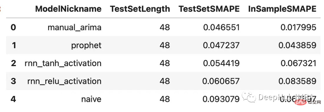
Now that we have generated predictions for each model, let’s see how they perform on the validation set, which we trained on The last 48 observations in the set.
results = f.export(determine_best_by='TestSetSMAPE')
 ms = results['model_summaries']
 ms[
[
 'ModelNickname',
 'TestSetLength',
 'TestSetSMAPE',
 'InSampleSMAPE',
]
 ]

Every model performed better than the naive method. The ARIMA model performed best with a percentage error of 4.7%, followed by the Prophet model. Let’s look at all the predictions versus the validation set:
f.plot(order_by="TestSetSMAPE",ci=True)
 plt.show()

All these models on this time series The performances are all reasonable, with no huge deviations between them. Let’s stack them up!
Stacked Models
Each stacked model requires a final estimator that will filter the various estimates from the other models to create a new set of predictions. We will overlay the previous results with the Catboost estimator. Catboost is a powerful program that hopefully fleshes out the best signal from each model that has been applied.
f.add_signals(
 f.history.keys(), # add signals from all previously evaluated models
 )
 f.add_ar_terms(48)
 f.set_estimator('catboost')
The code above adds the predictions from each evaluated model to a Forecaster object. It calls these predictions "signals." They are treated the same as any other covariates stored in the same object. The last 48 series of lags are also added here as additional regressors that the Catboost model can use to make predictions. Now let's call three Catboost models: one using all available signals and lags, one using only signals, and one using only lags.
f.manual_forecast(
 Xvars='all',
 call_me='catboost_all_reg',
 verbose = False,
 )
 f.manual_forecast(
 Xvars=[x for x in f.get_regressor_names() if x.startswith('AR')],
 call_me = 'catboost_lags_only',
 verbose = False,
 )
 f.manual_forecast(
 Xvars=[x for x in f.get_regressor_names() if not x.startswith('AR')],
 call_me = 'catboost_signals_only',
 verbose = False,
 )
The results of all models can be compared below. We will look at two metrics: SMAPE and mean absolute scaled error (MASE). These are two metrics used in actual M4 competition.
test_results = pd.DataFrame(index = f.history.keys(),columns = ['smape','mase'])
 for k, v in f.history.items():
 test_results.loc[k,['smape','mase']] = [
 metrics.smape(test_set,v['Forecast']),
 metrics.mase(test_set,v['Forecast'],m=24,obs=f.y),
]

 test_results.sort_values('smape')

可以看到,通过组合来自不同类型模型的信号生成了两个优于其他估计器的估计器:使用所有信号训练的Catboost模型和只使用信号的Catboost模型。这两种方法的样本误差都在2.8%左右。下面是对比图:
fig, ax = plt.subplots(figsize=(12,6))
 f.plot(
 models = ['catboost_all_reg','catboost_signals_only'],
 ci=True,
 ax = ax
 )
 sns.lineplot(
 x = f.future_dates,
 y = test_set,
 ax = ax,
 label = 'held out actuals',
 color = 'darkblue',
 alpha = .75,
 )
 plt.show()

哪些信号最重要?
为了完善分析,我们可以使用shapley评分来确定哪些信号是最重要的。Shapley评分被认为是确定给定机器学习模型中输入的预测能力的最先进的方法之一。得分越高,意味着输入在特定模型中越重要。
f.export_feature_importance('catboost_all_reg')

上面的图只显示了前几个最重要的预测因子,但我们可以从中看出,ARIMA信号是最重要的,其次是序列的第一个滞后,然后是Prophet。RNN模型的得分也高于许多滞后模型。如果我们想在未来训练一个更轻量的模型,这可能是一个很好的起点。
总结
在这篇文章中,我展示了在时间序列上下文中集成模型的力量,以及如何使用不同的模型在时间序列上获得更高的精度。这里我们使用scalecast包,这个包的功能还是很强大的,如果你喜欢,可以去它的主页看看:https://github.com/mikekeith52/scalecast
本文的数据集是M4的时序竞赛:https://github.com/Mcompetitions/M4-methods
使用代码在这里:https://scalecast-examples.readthedocs.io/en/latest/misc/stacking/custom_stacking.html
The above is the detailed content of Integrating time series models to improve forecast accuracy. For more information, please follow other related articles on the PHP Chinese website!
Related articles
See more- Technology trends to watch in 2023
- How Artificial Intelligence is Bringing New Everyday Work to Data Center Teams
- Can artificial intelligence or automation solve the problem of low energy efficiency in buildings?
- OpenAI co-founder interviewed by Huang Renxun: GPT-4's reasoning capabilities have not yet reached expectations
- Microsoft's Bing surpasses Google in search traffic thanks to OpenAI technology

