Application of causal inference in micro-view incentives and supply and demand scenarios

1. Causal inference and incentive algorithm

1. Business background and business modeling

First of all, let’s briefly introduce the background of Tencent Weishi’s red envelope incentive business. Similar to other products and scenarios, within a given budget, we issue some cash incentives to users of Tencent Weishi, hoping to maximize users’ next-day retention and usage time on the same day through cash incentives. The main form of cash incentives is to issue cash red envelopes of an indefinite number and an indefinite amount to users at irregular intervals. The three "uncertainties" mentioned above are ultimately determined by algorithms. These three "uncertainties" are also called the three elements of the red envelope incentive strategy.

# Next let’s talk about the abstract forms of different cash incentive strategies. The first one expresses the strategy in the form of a red envelope sequence, such as numbering the red envelope sequence, and then numbering each treatment independently in the form of one-hot. Its advantage is that it can depict more details, such as the amount between each red envelope and other detailed strategies, as well as the corresponding effects. However, this will inevitably require more variables to represent the strategy. The exploration space of the strategy is very large. In addition, more calculations will be required when exploring and selecting the strategy. The second form, which uses a three-element vector to represent the strategy, is more flexible and more efficient in exploration, but it does ignore some details. The third way is more mathematical, that is, the red envelope sequence directly becomes a function about time t, and the parameters in the function can form a vector to represent the strategy. The modeling of causal problems and the representation of strategies greatly determine the accuracy and efficiency of causal effect estimation.

Assuming that we have a good strategy abstraction and vector representation, the next thing to do is to choose an algorithm framework. There are three frameworks here. The first framework is relatively mature in the industry, which uses causal inference combined with multi-objective constraint optimization to allocate and optimize strategies. In this framework, causal inference is mainly responsible for estimating the core user indicators corresponding to different strategies, which is what we call user retention and duration improvement. After estimation, we use multi-objective constrained optimization to perform offline budget strategy allocation to satisfy the budget constraints. The second type is offline reinforcement learning combined with multi-objective constraint optimization method. I personally think this method is more promising for two main reasons. The first reason is that in actual application scenarios, there are many strategies, and reinforcement learning itself can efficiently explore the strategy space. At the same time, because our strategies are dependent, reinforcement learning can model the dependence between strategies; The second reason is that the essence of offline strong chemistry is actually a problem of counterfactual estimation, which itself has strong causal properties. Unfortunately, in our scenario, we have tried the offline reinforcement learning method, but its online effect did not achieve the desired effect. The reason is, on the one hand, our method problem, and on the other hand, it is mainly limited by the data. In order to train a good offline reinforcement learning model, the strategy distribution in the data needs to be wide enough, or the strategy distribution is uniform enough. In other words, whether we use random data or observational data, we hope to explore as many such strategies as possible, and the distribution will be relatively even, so that we can reduce the number of counterfactuals. The estimated variance. The last algorithm framework is relatively mature in advertising scenarios. We use online reinforcement learning to control traffic and budget. The advantage of this method is that it can respond to online emergencies in a timely and rapid manner, and at the same time, it can control the budget more accurately. After the introduction of cause and effect, the indicator we use for traffic selection or control is no longer the ECPM indicator. It may be an improvement in the retention and duration we estimate now. After a series of practical attempts, we finally chose the first algorithm framework, which is causal inference combined with multi-objective constraint optimization, because it is more stable and controllable, and it also relies less on online engineering.

The Pipeline of the first algorithm framework is shown in the figure below. First, user characteristics are calculated offline, and then a causal model is used to estimate the improvement of core indicators of users under different strategies, which is the so-called uplift. Based on the estimated improvement, we use multi-objective optimization to solve and assign the optimal strategy. In order to speed up the calculation of the entire process, we will cluster the crowd in advance when structuring, which means that we believe that the people in this cluster have the same cause and effect, and accordingly, we assign the same strategy to the people in the same cluster.

2. Strategy hypothesis and cause-and-effect diagram

Based on the above discussion, let’s focus on how to abstract the strategy. First let’s look at how we abstract the causal diagram. The cause and effect that needs to be modeled in the red envelope incentive scenario is reflected in multiple days and multiple red envelopes. Because the previous red envelope will definitely affect whether the next red envelope is received, it is essentially a Time-Varying Treatment Effect problem, abstracted into a time series causal diagram as shown on the right.

Take multiple red envelopes in one day as an example. All subscripts of T represent a serial number of the red envelope. T at this time represents the vector consisting of the amount of the current red envelope and the time interval since the last red envelope was issued. Y is the user's usage time after the red envelope is issued, and the increase in retention the next day. X is the confounding variable observed up to the current moment, such as the user's viewing behavior or demographic attributes, etc. Of course, there are many unobserved confounding variables, represented by U, such as users’ occasional stays or occasional stops. An important unobserved confounding variable is the user's mind, which mainly includes the user's value assessment of the amount of red envelope incentives. These so-called minds are difficult to represent through some statistical quantities or statistical characteristics within the system.

It would be very complicated to model the red envelope strategy in the form of time series, so we have made some reasonable simplifications. For example, assume that U only affects T, X and Y at the current moment, and it only affects U at the next moment, that is, the user's mind. That is to say, it will only affect the future Y by affecting the value evaluation or mentality of the next moment. But even after a series of simplifications, we will find that the entire time series causal diagram is still very dense, making it difficult to make reasonable estimates. And when using G-methods to solve the time Varying Trend Effect, a large amount of data is required for training. However, in reality, the data we obtain is very sparse, so it is difficult to achieve a good effect online. So in the end we made a lot of simplifications and got the fork structure (Fork) like the picture on the lower right. We made an aggregation of all red envelope strategies for the day, which is a vector composed of three elements of the strategy (total amount of red envelope incentives, total time, and total number), represented by T. X is a confounding variable at time T-1, which is the user’s historical behavior and demographic attributes as of that day. Y represents the user's usage time on that day, which is the user's retention or usage time indicator for the next day. Although this method seems to ignore many details, such as the interaction between red envelopes. But from a macro perspective, this strategy is more stable and its effects can be better measured.

3. Strategy representation and causal model

Based on the above discussion, the next step is the core issue, that is, how to express the strategy (treatment). Previously we tried using One-Hot to number the three-element vectors independently, and to separate the three elements and use the time function to construct a multi-variable treatment. The first two strategies are easier to understand, and the last method will be introduced next. Look at the picture above. We constructed the sine functions of the three elements with respect to t respectively, that is, given a time T, we can obtain the amount, time interval and number respectively. We use the parameters corresponding to these functions as elements of the new vector, similar to the representation of the three elements of the strategy. The purpose of using a function to represent the strategy is to retain more details, because the first two methods can only know the average amount of red envelopes and distribution intervals through a combination of strategies, and using a function may represent it in more detail. However, this method may introduce more variables, making the calculation more complex.

After having the strategy representation, we can select a causal model to estimate the causal effect. In the form of One-Hot representing the three elements of T, we use the x-Learner model to model each strategy, and use the strategy with the smallest total amount as the baseline strategy to calculate and evaluate the treatment effect of all strategies. In this case, you may feel that its efficiency is very low and the model lacks generalization. Therefore, we further adopt the third strategy just mentioned, that is, using a vector of sinusoidal function elements to form a treatment. A single DML model is next used to estimate the performance of all strategies relative to the baseline strategy. In addition, we also made an optimization DML, assuming that y is a linear weighting of the confounding variable and the causal effect, that is, y is equal to the treatment effect plus the confounding variable. In this way, the intersection terms and higher-order terms between vector elements are artificially constructed. It is equivalent to constructing a polynomial kernel function to introduce nonlinear functions. On this basis, DML has greatly improved compared to the baseline strategy. From the analysis of the figure below, we can find that the DML model costs less money and improves ROI, which means that we can use resources more efficiently.

Earlier we mainly discussed some method abstractions and model selection. During the practice process, we will also find some more business-oriented issues, such as What should I do about treatment when doing One-Hot? At this time, we implemented a batch-by-batch expansion strategy. First, make a seed strategy through the three elements of the strategy, and then manually screen and retain high-quality seeds, and then expand it. After expansion, we will launch new strategies in batches based on a period of time, such as the first two weeks of launch, and ensure that the random traffic size of each strategy is consistent or comparable. In this process, the impact of time factors will indeed be ignored, and less effective strategies will be continuously replaced, thereby enriching the collection of strategies. In addition, the time factor will definitely affect whether random traffic strategies are comparable. Therefore, we constructed a method similar to time slice rotation to ensure that the time slices covered are consistent, thereby eliminating the impact of time factors on the strategy, so that the random traffic obtained can be used to train the model.

#And how to generate a new strategy? A simple method is to use grade search, or genetic algorithm. These are more common general algorithms for search. In addition, we can combine manual pruning, such as cutting out some undesirable red envelope sequence types. Another method is to use BanditNet, which is an offline reinforcement learning method to calculate unseen strategies, that is, estimate the counterfactual effect, and then use the estimated value to make strategy selection. Of course, we will eventually need to use online random traffic to verify it. The reason is that the variance of this offline reinforcement learning method will probably be very large.

4. Strategic issues and iteration

In addition to the problems mentioned above, we will also encounter some business-oriented problems. The first question is what is the update cycle of user policies? Would it be better if all user policies were updated frequently? In this regard, our practical experience varies from person to person. For example, strategies for high-frequency users should change more slowly. On the one hand, this is because high-frequency users are already familiar with our format, including the incentive amount. If the red envelope amount changes drastically, it will definitely affect the corresponding indicators. Therefore, we actually maintain a weekly update strategy for high-frequency users, updating once a week; but for new users, the update cycle is shorter. The reason is that we know very little about new users, and we want to be able to explore appropriate strategies more quickly and respond quickly to make strategy changes based on user interactions. Since the behavior of new users is also very sparse, in this case, we will use the daily level to update new users or some low-frequency users. In addition, we also need to monitor the stability of the strategy to avoid the impact of feature noise. The Pipeline we built is shown on the right. Here we will monitor whether the treatment effect is stable, and we will also monitor the final strategy assigned by the user on a daily basis, such as the difference between today's strategy and yesterday's strategy, including the amount and number. We will also take regular snapshots of the online strategy, mainly for debugging and quick playback to ensure the stability of the strategy. In addition, we will also conduct experiments on small traffic and monitor its stability. Only small traffic experiments that meet stability requirements will be used to replace existing strategies.

#The second question is whether the policies for new users and some special users are independent? The answer is yes. For example, for new users, we will first provide him with a strong incentive, and then the intensity of the incentive will decay over time. After the user enters the normal life cycle, we will implement regular incentive strategies for him. At the same time, for special sensitive groups, there will be a restriction policy on their amount. For this, we will also train independent models to adapt to this group of people.

The third question you may ask is, how important is causal inference in the entire algorithm framework? From a theoretical perspective, we believe that causal inference is core because it brings great benefits in incentive algorithms. Compared with regression and classification models, causal inference is consistent with business goals and is inherently ROI-oriented, so it will bring optimization goals regarding the amount of improvement. However, we would like to remind everyone that when we allocate budgets, we cannot choose the optimal strategy for every user, and the causal effect is relatively small compared to individuals. When we allocate budgets, it is very likely that some differences in user causal effects will be eliminated. At this time, our constrained optimization will greatly affect the strategy effect. Therefore, when doing clustering, we also tried more clustering methods, such as the deep clustering SCCL method to obtain better clustering results. We have also carried out some iterations of deep causal models, such as BNN or Dragonnet, etc.

We found that during practice, the offline indicators of the deep causal model have indeed improved significantly, but its online effect is not stable enough. The reason is that there are missing values. At the same time, we also found that the feature planning method greatly affects the stability of the deep learning online model, so in the end we will tend to use the DML method stably.

# So much for sharing in the incentive scenario. Next, I would like to ask two other students from our team to share with you some practices in the supply and demand optimization scenario. and theoretical exploration.

2. Causal inference and supply and demand adjustment

1. Business background and business modeling

Next Let me introduce the business background of Tencent Weishi in terms of supply and demand. As a short video platform, Weishi has many different categories of videos. For user groups with sometimes different viewing interests, we need to appropriately allocate the exposure proportion or inventory proportion of each category according to different user characteristics. The goal is to improve the user experience and user viewing time, among which the user’s The experience can be measured based on the 3-second fast-swipe rate indicator, and the viewing time is mainly measured based on the total playback time. How to adjust the exposure ratio or inventory ratio of video categories? Our main consideration is to increase or decrease some categories in proportion. The ratio of increase and decrease is a preset value.

Next we need to use algorithms to solve how to decide which categories to increase and which categories to decrease, so as to maximize the user experience and viewing time, and at the same time, we need to meet the requirements For example, there are some constraints that limit the total exposure. This place summarizes three main modeling ideas. The first is a more direct idea, that is, we directly treat the increase and decrease as a treatment variable of 0 and 1, we estimate its causal effect, and then conduct a multi-objective constrained optimization to Get a final strategy. The second idea is to model treatment more carefully. We treat treatment as a continuous variable. For example, the exposure ratio of a category is a variable that changes continuously between 0 and 1. Then fit a corresponding causal effect curve or causal effect function, and then perform multi-objective constrained optimization, and finally obtain the final strategy. It can be noted that the two methods just mentioned are two-stage methods. The third idea, We bring constraints into the estimation of causal effects, thereby obtaining an optimal strategy that satisfies the constraints. This is also the research content I hope to share with you later.

First of all, let’s focus on the first two modeling ideas. There are several modeling points that need to be paid attention to. The first point is that in order to ensure the accuracy of causal effect estimation, we need to divide the population and estimate the causal effect of binary treatment or continuous treatment on each population. Just now, Teacher Zheng also mentioned methods of classifying people, such as using Kmeans clustering or some deep clustering. The second point is how to evaluate the model effect on non-random experimental data. For example, we need to evaluate the effect of the model offline without doing AB test. Regarding this issue, you can refer to some indicators mentioned in the paper indexed above in the PPT for offline evaluation. The third point to note is that we should consider the correlation and mutual influence between categories as much as possible, such as some problems of crowding out between similar categories, etc. If these factors can be included in the estimation of causal effects, better results should be achieved.

##2. Single group × category exposure proportion adjustment strategy

Next we will expand on these modeling ideas in detail. First of all, the first modeling method is to define a treatment of 0 and 1, which is used to represent the means of increasing or decreasing these two types of intervention. You can refer to the brief cause-and-effect diagram on the left. Here x represents some characteristics of the user, such as historical operation behavior. Relevant statistical characteristics, as well as other user attributes, etc. y is the target we care about, which is the 3-second acceleration rate or the total playback time. In addition, it is also necessary to pay attention to some unobserved confounding variables, such as users' accidental, fast swiping and exit, and the same user may actually be used by multiple people, which is also a problem of multiple identities of users. In addition, the continuous iteration and update of the recommendation strategy will also have an impact on the observation data, and the migration of user interests is also outside the observation. These unobserved confounding variables may affect the estimation of causal effects to a certain extent.

For such a modeling method, common causal effect estimation methods can be solved. For example, you can consider T-Learner or X-Learner, or DML, which can estimate causal effects. Of course, this simple modeling method also has some problems. For example, if we use binary treatment to model, it will be too simplified. In addition, under this method, each category is considered separately, and the correlation between categories is not considered. The last problem is that we did not consider specific factors such as the order of exposure and the quality of the content in the entire question.

# Next, let’s introduce the second modeling idea. We consider all categories together. For example, we have k video categories, and let treatment be a k-dimensional cause vector. Each position of the vector represents a category, such as film and television variety shows or MOBA events, etc. 0 and 1 still represent increases or decreases. At this time, the causal effect estimation of treatment in multi-dimensional vectors can be solved by DML algorithm. We usually treat the treatment vector, which is all 0, as the control. Although this method solves the problem that each category is not considered separately, it still has some potential problems. The first is the problem of dimensionality explosion caused by too many categories. As the dimensions increase, since there are two situations of 0 and 1 at each position, the number of potential permutations and combinations will increase exponentially, which will affect the cause and effect. The accuracy of effect estimates creates interference. In addition, factors such as the exposure sequence and content mentioned earlier are not taken into account.

After sharing the modeling ideas of the binary variable treatment, we can next Carry out more detailed modeling that is more in line with its own characteristics. We noticed that the exposure ratio itself is a continuous variable, so it is more reasonable for us to use continuous treatment for modeling. Under this modeling idea, we first need to divide the crowd. For each group of people, we model each category separately and obtain a causal effect curve of a single group*single category. As shown in the picture on the left, the causal effect curve represents the impact of the proportion of different categories on the goals we care about. In order to estimate such a causal effect curve, I mainly share two feasible algorithms, one is DR-Net and the other is VC-Net. Both algorithms belong to the category of deep learning. The structure of the model is as shown in the picture on the right.

First introduce DR-Net. The input x of the model will first go through several fully connected layers to obtain an implicit representation called z. DR-Net adopts a discretization strategy, which disperses the continuous treatment into multiple blocks, and then each block trains a sub-network to predict the target variable. Since DR-Net adopts a discretization strategy, the final causal effect curve it obtains is not strictly continuous, but as the discretization becomes thinner, the final estimate will be closer to a continuous curve. Of course, as the idealized segmentation becomes thinner, it will bring more parameters and a higher risk of overfitting.

Next I will share about VC-Net. VC-Net improves the shortcomings of DR-Net to a certain extent. First of all, the input of the VC-Net model is still X, which is also the user's characteristic. It also first obtains an implicit representation Z after several fully connected layers. But at Z, a module for predicting Propensity Score will be connected first. Under continuous Treatment conditions, Propensity is a probability density of Treatment t under a given X condition, which is also π represented on the figure. Next, let's take a look at the network structure after Z. Unlike DR-Net's discretization operation, VC-Net uses a variable coefficient network structure, that is, each model parameter after Z is a parameter about t The function. The authors of the literature we mentioned here used the basis function method to express each function as a linear combination of basis functions, which is also written as θ (t). In this way, the estimation of the function becomes the parameter estimation of the linear combination of the basis functions. So in this way, the parameter optimization of the model is not a problem, and the causal effect curve obtained by VC-Net is also a continuous curve. About the objective function to be solved by VC-Net consists of several parts. On the one hand, it consists of the squared loss of the final prediction on the target, which is μ in the figure. On the other hand, it also consists of the logarithmic loss of the probability density of propensity. In addition to these two parts, the author also adds a penalty term called targeted regularization to the objective function, so that double robust estimation properties can be obtained. For specific details, interested friends can refer to the two original papers indexed above for more details.

Finally, let’s pave the way for a piece of our research that we will share with you soon. . We noticed that the exposure proportion of each video category is a multi-dimensional continuous vector. The reason why it is multi-dimensional is that we have multiple video categories, and each dimension represents a video category. The main reason why it is continuous is that the exposure proportion of each video category is continuous, and its values ​​are between 0 and 1. At the same time, there is a natural constraint, which is that the total exposure ratio of all our video categories must be equal to 1. So we can consider such a multi-dimensional continuous vector as treatment.

#The vector shown on the right is an example of this. Our goal is to find the optimal exposure ratio to maximize our total play time. In the traditional causal framework, it is difficult for algorithms to solve such a multi-dimensional continuous and unconstrained problem. Next, we share our research on this issue.

##3. Sharing of Constrained Continuous Multivariable Causal Model

MDPP Forest This work is a method exploration and innovative solution to the problem done by the team when studying supply and demand issues. Our team discovered at that time that when faced with the problem of how to allocate the best video category exposure ratio for each user, other existing common methods could not achieve a result that was more in line with expectations. Therefore, after a period of trial and improvement, the method designed by our team can achieve good results offline, and then cooperate with recommendations, and finally achieve certain strategic benefits. We then compiled this work into a paper, which was fortunate enough to be published on KDD 2022.

## 1. Background and challenges

First, introduce the background of the problem. In terms of supply and demand, we divide short videos into different categories based on content, such as popular science, film and television, outdoor food, etc. The video category exposure ratio refers to the proportion of each of these different categories of videos among all the videos watched by a user. Users have very different preferences for different categories, and platforms often need to determine the optimal exposure ratio for each category on a case-by-case basis. In the re-ordering stage, the recommendation of various types of videos is controlled. A big challenge for the company is how to allocate the best ratio of video exposures to maximize each user's time on the platform.

#The main difficulty with such a problem lies in the following three points. The first one is that in the short video recommendation system, the videos that each user sees have a very strong correlation with his own characteristics. This is a selective bias. Therefore, we need to use algorithms related to causal inference to eliminate bias. The second is that the video category exposure ratio is a continuous, multi-dimensional and constrained treatment. There are currently no very mature methods for such complex problems in the fields of causal inference and policy optimization. The third is that in offline data, we cannot know a priori the true optimal exposure ratio of each person, so it is difficult to evaluate this method. In a real environment, it is only a sub-link in recommendation. The final experimental results cannot judge the accuracy of this methodfor its own calculation goals. Therefore, it is difficult for us to accurately evaluate the problem of this scenario. We will introduce how we conduct effect evaluation later.

2. Problem Definition

We First, abstract the data into a causal diagram in statistics. Among them, vector. Y is the user’s viewing time, which is the response to the task goal. The goal of our modeling is to give a high-dimensional optimal video category exposure ratio under specific user characteristics X, so as to maximize the user's viewing time expectation. This problem seems to be simply represented by a causal ternary diagram, but there is a big problem, which is mentioned earlier. Our treatment is the exposure ratio of multiple categories, which is accounted for by category exposure. Ratio constructs a multi-dimensional vector with continuous values ​​and the sum of the vectors is 1. This problem is more complicated.

##3. Method introduction——Maximum Difference Point of Preference (MDP2) Forest

In this regard, our method is also based on the causal forest (causal forest). General causal decision trees can only solve treatment problems with one-dimensional discrete values. By improving the calculation of the intermediate split criterion function, we add some high-dimensional continuous information during splitting, so that it can solve the problem of high-dimensional continuous values ​​and constrained treatment.

##① Introduction to the method - continuous problem

First, we solve the problem of continuous treatment. As shown in the figure, the effect of T on Y is a continuous curve. Let's first assume that this is a monotonically increasing curve. For all Treatment values ​​in the data, we traverse it and calculate the Y mean of the left and right samples to find the point with the largest difference between the Y mean on the left and the Y mean on the right, that is, the point with the largest average causal benefit. We call this point the Maximum Difference Point, which is the most efficient point on the continuous Treatment space, which means that the Treatment can significantly change Y. Maximum Difference Point is the point we want to get in a single dimension.

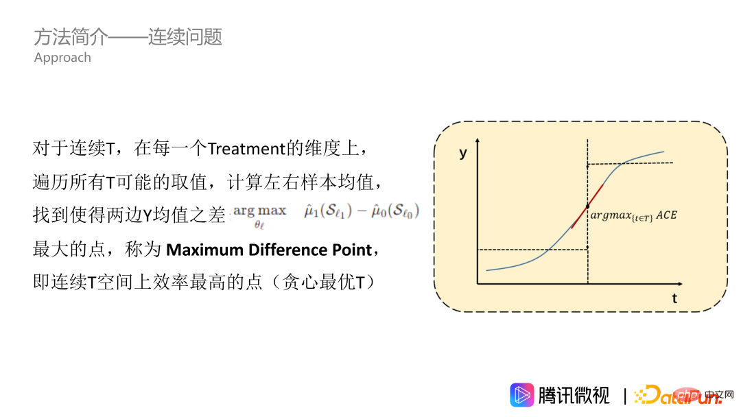
However, the method we just mentioned is only suitable for monotonically increasing curves. But in fact, most problems are not so good, especially the issue of exposure ratio. On this issue, the effect curve is generally mountain-shaped, that is, it increases first and then decreases. Recommending more videos that users like can increase the viewing time of users. However, if this type is recommended too much, the entire video recommendation will become very monotonous and boring, and it will also crowd out the exposure space of video types that other users like. So the curve is generally mountain-shaped, but it may also be in other shapes. In order to adapt to the T-curve of any shape, we need to perform an integral operation, that is, to find the value range interval for accumulation. On the accumulated curve, we also calculate the mean values ​​on the left and right sides, as well as the point where the difference between the mean values ​​on the two sides is the largest, such as the five-pointed star in the picture. This point can be called the maximum difference point of preference, which is our MDPP.

② Introduction to the method - high-dimensional problem

We introduced how to solve the continuous problem above, but the curve just mentioned is only one-dimensional and corresponds to a single video category. Next, we use the idea of ​​heuristic dimension traversal to solve multi-dimensional problems. When calculating the classification score, we use a heuristic idea to randomly sort the K dimensions, and calculate an aggregation of D indicators in each dimension, that is, perform a summation operation. Obtain D* as a high-dimensional information entropy, and then consider the constraint. The constraint is that the sum of all MDPPs is 1. Here we have to consider the following two situations. One is if the sum of MDPP does not reach 1 after the K dimension is traversed. In response to this situation, we will add the sum of all MDPPs and normalize them to 1. The second case is that if we only traverse the K' dimension, which is smaller than the K dimension, the sum of MDPP has reached 1. For this, we will stop the traversal and set the MDPP to the remaining "resource amount", which is 1 minus the sum of the previously calculated MDPP values, so that the constraints can be taken into account.

In addition, we will also introduce forest to the above tree structure, because it mainly There are two major meanings. The first is our traditional bagging ensemble idea, which can use multiple learners to enhance the robustness of the model. The second is that in dimension traversal, only K’ dimensions will be calculated each time a node is split, and some dimensions are not included. In order for each dimension to have an equal chance to participate in the split, we need to build multiple trees.

③ Method introduction-algorithm acceleration

There is another problem. Since the algorithm contains three levels of traversal, all tree models require eigenvalue traversal, as well as additional dimension traversal and MDPP search traversal. Such three-layer traversal makes the efficiency very low. Therefore, we use the weighted quantile graph method for eigenvalue traversal and MDPP traversal, and only calculate the corresponding results at the quantile points, which can greatly reduce the algorithm complexity. At the same time, we also found these quantile points as the boundary points of the "cumulative value range", which can greatly reduce the amount of calculation and storage. Assuming there are q quantiles, we only need to calculate q times to get the number of samples and the mean value of y in each quantile interval. In this way, every time we calculate the difference d between the means on both sides, we only need to divide the q value into the left For the two parts on the right, just do a weighted sum of the average values ​​in each interval. We no longer need to recalculate the mean of all samples to the left and right of the quantile point. Let’s enter the experimental part below.

4. Experimental design

① Experimental design-Metric

Our experimental evaluation is essentially a strategy Evaluation problem, so we introduce indicators related to strategy evaluation. The first is the Main Regret, which measures the gap between the overall strategy's return and the theoretical optimal return. The other is Main Treatment Square Error, which is used to measure the gap between the estimated value and the optimal value of each Treatment dimension under multi-dimensional Treatment. For both indicators, the smaller the better. However, the biggest problem caused by setting these two evaluation indicators is how to determine the optimal value.

##② Experimental Design-Contrast Method

Introduce our comparison method. The first is two commonly used methods in causal inference, one is DML with complete statistical theory, and the other is the network model DR-Net and VC-Net. These methods can only handle one-dimensional problems, but for the problem in this article, we have made some adjustments to deal with multi-dimensional problems, that is, first calculate the absolute value of each dimension and then perform normalization. There are also strategy optimization methods in the following two papers, which we call OPE and OCMD. These two articles state that their methods are suitable for multidimensional problems, but they also point out that when there are too many dimensions, it is difficult for these methods to be effective.

##③ Experimental design-simulation data set

In order to compare model effects simply and directly, we simulated real-world problems and generated a simplified version of the simulation data set. The feature space x represents 6 dimensions of user features and 2 behavioral features. For samples with different characteristics, we first assume its optimal strategy. As shown in the figure, for example, a user who is younger than 45 years old, has an education level greater than 2, and has a behavioral characteristic greater than 0.5 is the best in 6 video categories. With the help of the formula on the left, first randomly generate an exposure strategy for the user, and then calculate the gap between the exposure strategy and the real optimal strategy, as well as the duration of the simulated user. If the strategy is closer to the user's optimal strategy, the user's duration y will be longer. In this way we generated such a data set. The advantage of this simulated data set is that we directly assume the optimal value, which is very convenient for evaluation. The other is that the data is relatively simple, which makes it easier for us to analyze the results of the algorithm.

Let’s take a look at the experimental results on the simulated data set. For what we just mentioned For that type of population, various methods are provided to calculate the mean value of the corresponding treatment. The first line is the theoretical optimal, the second line is our MDPP forest, and the third line is based on MDPP forest and adds some penalty terms to the splitting criterion. It can be seen that the gap between our method and the theoretical optimal will be very small. The other methods are not particularly extreme, but are relatively even. In addition, from the MR and MTSE figures on the right, our two methods also have very obvious advantages.

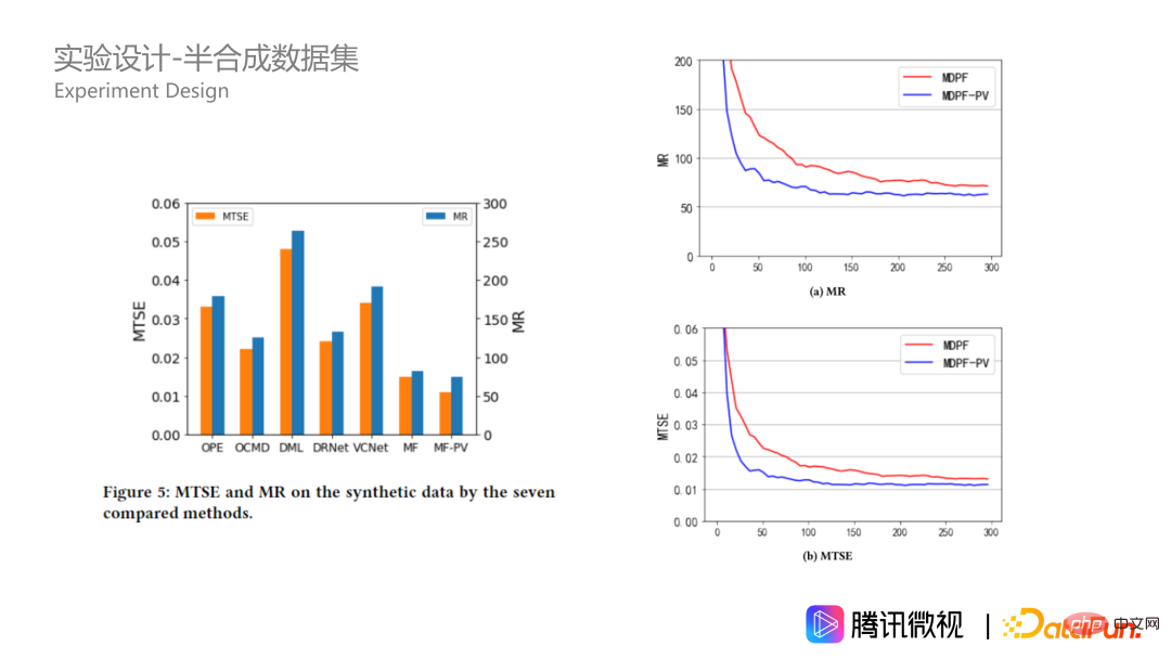
④ Experimental design-semi-synthetic data set

In addition to the simulated data set, we also constructed a semi-synthetic data based on real business data. The data comes from Tencent Weishi platform. Xi represents the 20-dimensional characteristics of the user, treatment ti represents the multi-dimensional video category exposure ratio forming a 10-dimensional vector, and yi(ti) represents the usage time of the i-th user. One characteristic of actual scenarios is that we cannot know the user's real optimal video exposure ratio. Therefore, we construct a function according to the cluster center rules and generate virtual y to replace the real y, so that the y of the sample has better regularity. I won’t go into details about the specific formula here. Interested students can read the original text. Why is this possible? Because the key to our algorithm is that it must be able to resolve some confounding effects between x and t, that is, online users are affected by biased strategies. In order to evaluate the effect of the strategy, we only keep x and t and change y to better evaluate the problem.

On semi-synthetic data, our algorithm also performs significantly better and is better than The advantages on simulated data sets will be even greater. This shows that our MDPP forests algorithm is more stable when the data is complex. In addition, let's take a look at the hyperparameters on synthetic data, which is the size of the forest. In the picture on the lower right, we can see that as the forest size increases, the indicators converge better under the two splitting criteria. The one with the penalty term will always be better, and it reaches better when there are 100 trees. The optimal effect is achieved with 250 trees, and then there will be some overfitting.

4. Q&A session

Q: Why traverse Can normalization work when the exposure exceeds 1?

#A: My understanding is this, because what we are doing is an optimization of exposure proportion constraints. In this process, we are a relative value. In the process of traversing, we are looking for the optimal split point and finding which category should be given priority and the proportion of exposure. In this process, as long as we can ensure that it is proportionally scaled, it is okay.

#I have the same view, it can be scaled proportionally. Because 1 is a strong constraint, the value we calculated at the beginning will definitely not be exactly 1, but will be lower or higher. If there are a lot more, there is no way to make it meet the unique condition of strong constraints, and it is more natural to use a normalized thinking. Because we consider the relative size relationship between each category. I think the relative size relationship is more important, rather than a question of absolute value.

The above is the detailed content of Application of causal inference in micro-view incentives and supply and demand scenarios. For more information, please follow other related articles on the PHP Chinese website!