Five commonly used loss functions for training deep learning neural networks

The optimization of neural network during training is to first estimate the error of the current state of the model, and then in order to reduce the error of the next evaluation, it is necessary to use a function that can represent the error to update the weight. This function is called a loss function.

#The choice of loss function is related to the specific predictive modeling problem (such as classification or regression) for which the neural network model learns from examples. In this article we will introduce some commonly used loss functions, including:

• Mean square error loss of regression model
• Cross entropy and hinge loss of binary classification model

Loss function of regression model

The regression prediction model is mainly used to predict continuous values. So we will use scikit-learn's make_regression() function to generate some simulated data and use this data to build a regression model.

We will generate 20 input features: 10 of them will be meaningful, but 10 will be irrelevant to the problem.

And randomly generate 1,000 examples. And specify a random seed, so the same 1,000 examples are generated whenever you run the code.

Scaling real-valued input and output variables to a reasonable range often improves the performance of neural networks. So we need to standardize the data.

StandardScaler can also be found in the scikit-learn library. To simplify the problem we will scale all the data before splitting it into training and test sets.

Then split the training and validation sets equally

To introduce different loss functions, we will develop a small multi- Layer Perceptron (MLP) model.

According to the problem definition, there are 20 features as input, which pass through our model. A real value is required to predict, so the output layer will have a node.

We use SGD for optimization, and have a learning rate of 0.01 and a momentum of 0.9, both of which are reasonable default values. Training will be conducted for 100 epochs, the test set will be evaluated at the end of each stage, and the learning curve will be plotted.

After the model is completed, the loss function can be introduced:

MSE

The most commonly used regression problem is the mean square error loss. (MSE). It is the preferred loss function under maximum likelihood inference when the distribution of the target variable is Gaussian. So you should only change to other loss functions if you have a better reason.

If "mse" or "mean_squared_error" is specified as the loss function when compiling the model in Keras, the mean squared error loss function is used.

The code below is a complete example of the above regression problem.

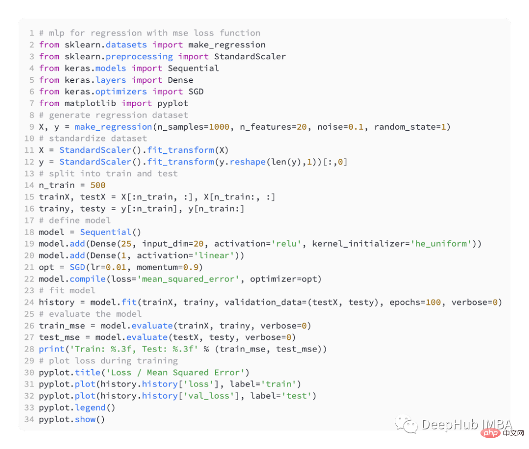
In the first step of running the example, the mean square error of the training and test data sets of the model is printed. Because 3 decimal places are retained, it is displayed as 0.000

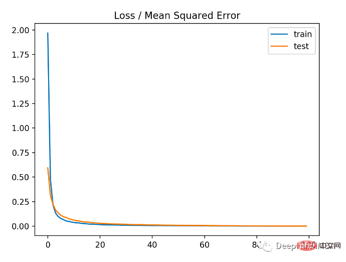
As you can see from the figure below, the model converges quite quickly and the training and testing performance remains unchanged. Depending on the performance and convergence properties of the model, mean square error is a good choice for regression problems.

#MSLE

In regression problems with a wide range of values, it may not be desirable to penalize the model as much as mean squared error when predicting large values. So the mean squared error can be calculated by first calculating the natural logarithm of each predicted value. This loss is called MSLE, or mean square log error.

It has the effect of relaxing the penalty effect when there is a large difference in the predicted values. It may be a more appropriate loss measure when the model directly predicts unscaled quantities.

Using "mean_squared_logarithmic_error" as the loss function in keras

The example below is the complete code using the MSLE loss function.

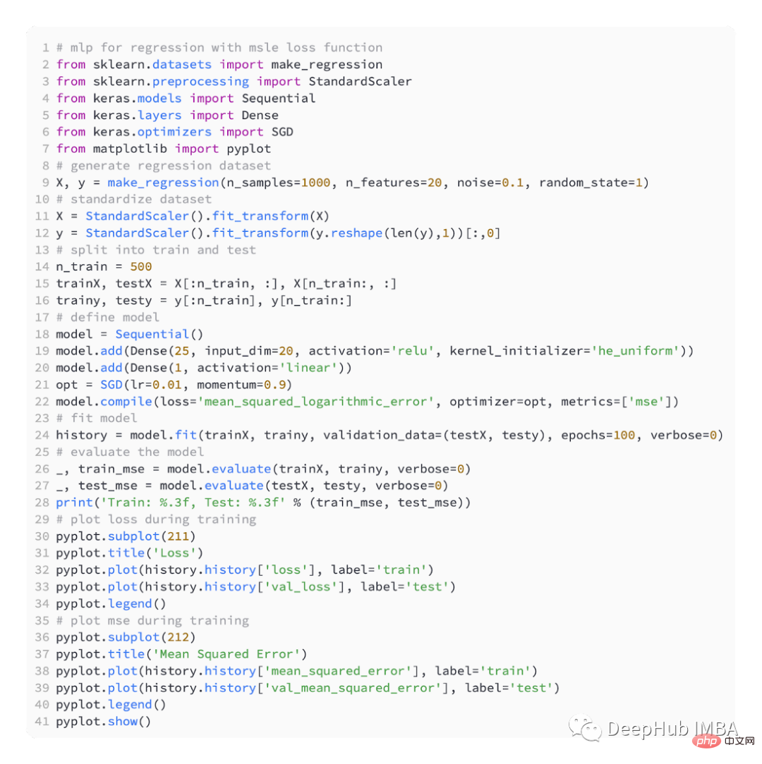
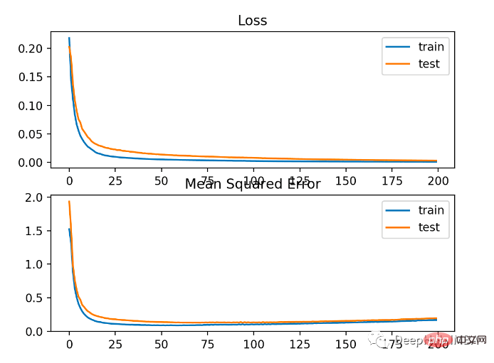
The model has slightly worse MSE on both the training and test datasets. This is because the distribution of the target variable is a standard Gaussian distribution, which means that our loss function may not be very suitable for this problem.

The figure below shows the comparison of each training round. The MSE converges well, but the MSE may be overfitting because it decreases from round 20 to change and starts to rise.

MAE

Depending on the regression problem, the distribution of the target variable may be mainly Gaussian, but may contain outliers, such as large values ​​far away from the mean or Small value.

In this case, the mean absolute error or MAE loss is a suitable loss function as it is more robust to outliers. Calculated as an average, taking into account the absolute difference between the actual and predicted values.

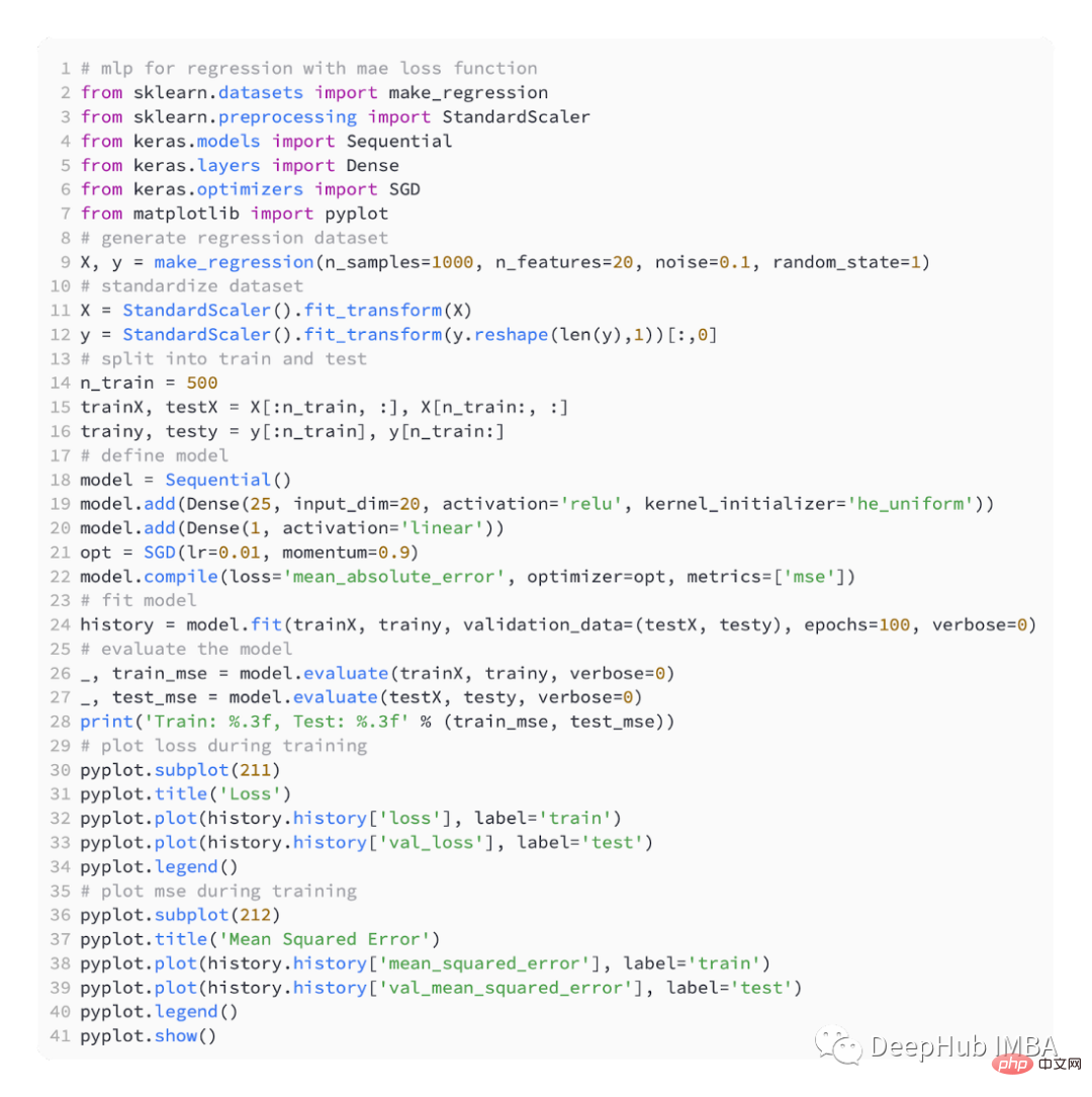
Using the "mean_absolute_error" loss function

This is the complete code using MAE

The result As shown below

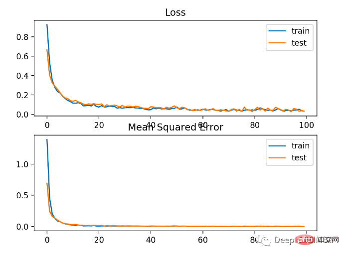
As you can see from the figure below, MAE has indeed converged but it has a bumpy process. MAE is also not very suitable in this case because the target variable is a Gaussian function without large outliers.

Loss function for binary classification

A binary classification problem is one of two labels in a predictive modeling problem. This problem is defined as predicting the value of the first or second class as 0 or 1, and is generally implemented as predicting the probability of belonging to the class value 1.

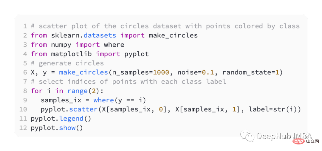
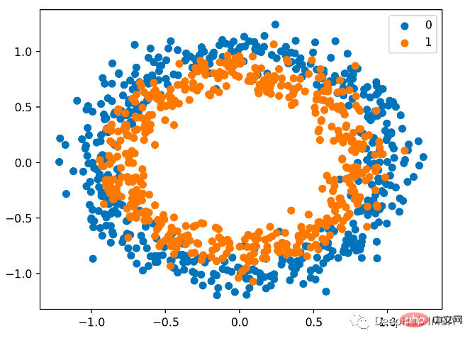
We also use sklearn to generate data. Here we use a circle problem. It has a two-dimensional plane and two concentric circles. The points on the outer circle belong to class 0 and the points on the inner circle belong to class 1. To make learning more challenging, we also add statistical noise to the samples. The sample size is 1000, and 10% statistical noise is added.

A scatter plot of a data set can help us understand the problem we are modeling. Listed below is a complete example.

#The scatter plot is as follows, where the input variables determine the location of the points, and the colors are class values. 0 is blue and 1 is orange.

Here is still half for training and half for testing.

We still define a simple MLP model ,

Use SGD optimization with a learning rate of 0.01 and a momentum of 0.99.

The model is trained for 200 rounds of fitting, and the performance of the model is evaluated based on loss and accuracy.

BCE

BCE is the default loss function used to solve binary classification problems. Under maximum likelihood inference framework, it is the loss function of choice. For predictions of type 1, cross-entropy calculates a score that summarizes the average difference between the actual and predicted probability distributions.

When compiling the Keras model, binary_crossentropy can be specified as the loss function.

#To predict the probability of class 1, the output layer must contain a node and a 'sigmoid' activation.

The following is the complete code:

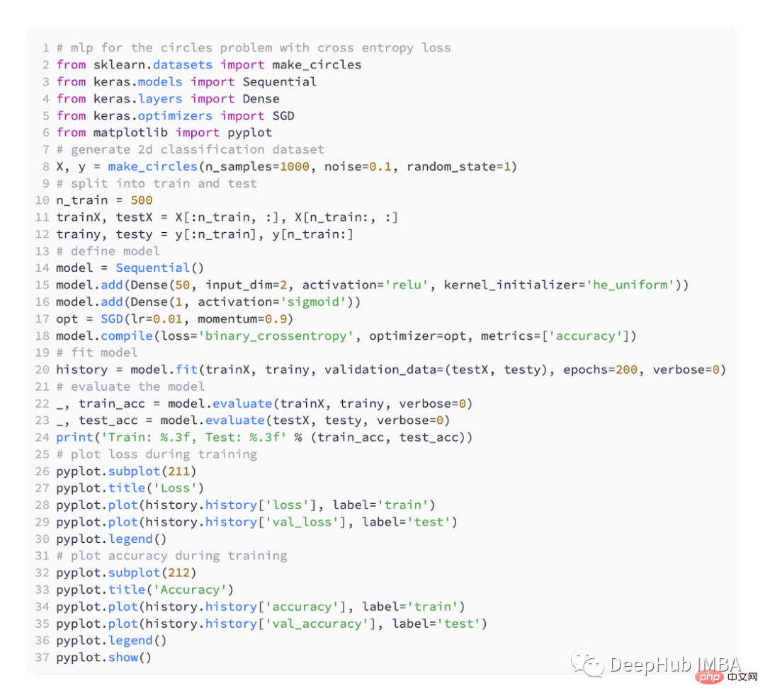
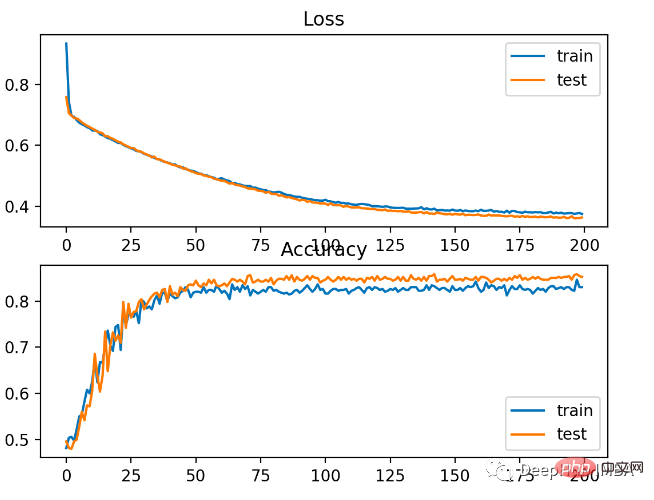
The model learns the problem relatively well, in the test data set The accuracy rate is 83% and the accuracy rate is 85%. There is some degree of overlap between the scores, indicating that the model is neither overfitting nor underfitting.

As shown in the picture below, the training effect is very good. Since the error between the probability distributions is continuous, the loss plot is smooth, while the accuracy line plot shows bumps because examples in the training and test sets can only be predicted as correct or incorrect, providing less granular information.

Hinge

The Support Vector Machine (SVM) model uses the Hinge loss function as an alternative to cross-entropy to solve binary classification problems.

The target value is in the set [-1, 1] , intended for use with binary classification. Hinge will get larger errors if the actual and predicted class values ​​have different signs. It is sometimes better than cross entropy on binary classification problems.

As a first step, we must modify the value of the target variable to the set {-1, 1}.

It is called ' hinge ' in keras.

In the output layer of the network, a single node with the tanh activation function must be used to output a single value between -1 and 1.

The following is the complete code:

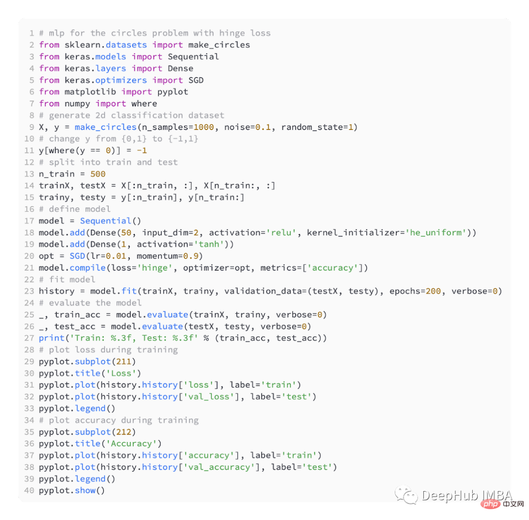
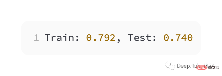
Slightly worse performance than cross entropy, on the training and test sets The accuracy is less than 80%.

#As can be seen from the figure below, the model has converged, and the classification accuracy graph shows that it has also converged.

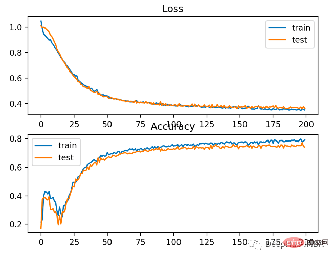
You can see that BCE is better for this problem. The possible reason here is that we have some noise points

The above is the detailed content of Five commonly used loss functions for training deep learning neural networks. For more information, please follow other related articles on the PHP Chinese website!