


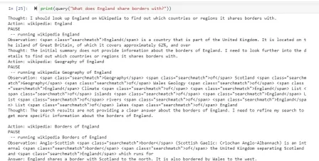
Summary of main technical ideas and methods of causal inference


Introduction: Causal inference is an important branch of data science and plays an important role in the evaluation of product iterations, algorithms and incentive strategies in the Internet and industry. Its role is to combine data, experiments or statistical econometric models to calculate the benefits of new changes, which is the basis for decision-making. However, causal inference is not a simple matter. First of all, in daily life, people often confuse correlation and causation. Correlation often means that two variables have a tendency to increase or decrease at the same time, but causation means that we want to know what will happen when we change a variable, or we expect to get a counterfactual result, if we did it in the past If we take different actions, will there be changes in the future? The difficulty, however, is that counterfactual data are often difficult to observe and collect in the real world.
This article reviews two schools of causal inference—Rubin Causal Model (RCM; Rubin 1978) and Causal Diagram (Pearl 1995) )'s main technical ideas and methods, as well as new methods and applications in recent years. Since the author's academic background is relatively related to econometrics, the methods and papers cited mainly refer to economic literature. There may be some omissions in the depth and breadth of the theory and application of some methods. Please forgive me.
Potential Outcome Model
We use i to represent each research object or user, and they may be subject to certain strategic intervention: Ti=1 represents the intervention (experimental group), Ti=0 represents no intervention (baseline group), and the corresponding results we care about are Yi0 and Yi1, but only one situation will actually happen, that is, Yi0 and Yi1Only one of them can be observed, and the other is unknown. The causal inference result we expect here is the average treatment effect ATE=E[Y1-Y0].
We can explain the difficulty of estimating ATE through certain mathematical derivation. Since we will only observe one of Yi0 and Yi1 , what we can directly calculate is actually the inter-group difference E[Yi1|T# between the experimental group and the baseline group ##i##=1]-E[Yi0|Ti =0], This difference can be further broken down to equal E[Yi1|Ti##=1]-E[Yi0|Ti=1] E[Yi0|T i=1]-E[Yi0|Ti=0]. Where E[Yi1|Ti=1]-E[ Yi0|T#i=1] is on the individual in the experimental group Average treatment effect (ATT), ATT and ATE are often not equal, and the difference between the two represents the external validity (External Validity) we calculate. If the sample is limited to users of a certain age group, the results may not be generalizable to users of all age groups, indicating that our analysis may not have external validity. The second part of the above formula E[Yi0|Ti =1]-E[Yi0|Ti=0] Represents sample selection bias. Selective bias may often not be 0 in real life. For example, if the experimental group and the benchmark group are not randomly sampled, and there will be differences in certain feature distributions, then selectivity bias may occur. Therefore, the difference between groups we calculate actually represents the average treatment effect we expect only when the selection bias is eliminated, has external validity, and is based on a large and sufficient sample. The thinking method of the potential effect model is actually to achieve such conditions through certain settings and models. Behind its ideas, there are also relatively strict mathematical assumptions. Below, we review the main ideas and the technological development and applications in recent years according to different methods. Due to space limitations, the breakpoint regression method will not be introduced in detail here. 1.
A/B testingThe most common method of potential effect model is Randomized experiments, or A/B testing that we commonly use in industry. We constructed the experimental group and the baseline group through certain random sampling to observe the differences between the groups. However, it should be pointed out that even if randomness is satisfied, the effectiveness of causal inference here still needs to meet an important assumption - Stable Unit Treatment Value Assumption (SUTVA). The potential outcomes of each individual are only relevant to himself and have nothing to do with whether other individuals are intervened by the experimental strategy. At the same time, the single strategic intervention we are concerned about does not have different forms or intensities that lead to different potential outcomes. In real life, there are many scenarios where SUTVA assumptions are violated, which has also inspired the development of various new A/B testing techniques, such as budget or strategic control for crowding problems, or improvements in diversion design. Here we give some examples related to diversion:
At LinkedIn, experimenters use network sampling experimental methods to deal with the challenges that social networks pose to traditional individual random experiments. First, users are divided into different clusters, and each cluster is used as an individual to randomly divide and measure experimental indicators. The estimated treatment effect is corrected by estimating the user's network effect exposure (Gui et al. 2015). On platforms such as Airbnb, there is often mutual influence between buyers and sellers, which can also interfere with traditional experimental methods. Researchers construct experimental evaluation indicators through bilateral experimental design and dynamic models of inventories (Johari et al. 2022). It should be pointed out that bilateral experiments are a relatively new field, and their experimental design can help experimenters discover the spillover effects of traditional unilateral experiments. However, it is difficult to make statistical inferences and corrections for experimental results, and there may not be an absolute answer. It should be discussed more in combination with business scenarios. ##Image from the paper Johari et al. (2022) Instrumental variable is a method to solve the endogeneity problem of linear regression. Next, we introduce the endogeneity problem and how to solve endogeneity through instrumental variables. The main problem with endogeneity is if we care about the effect of X on Y, but there is an unmeasured variable U that affects both X and Y. Then X is endogeneous, and U is the confounding variable mentioned above. If we can find a variable Z that is related to X, and Z is not related to U. Then we can use Z as an instrumental variable to estimate the causal effect of X on Y. The specific calculation method is generally the two-stage least squares method. When the instrumental variable method is actually used, attention should be paid to avoiding the problem of "weak instrumental variables", that is, the correlation between the instrumental variable Z and the variable of interest X is very low, which will cause bias in the estimated causal effect. Statistical testing methods can be relied on. to confirm whether such a problem exists. One development of the instrumental variable method is to combine it with a deep learning model, for example, proposed by Hartford et al. (2017) Deep IV method. This research transforms the traditional two-stage least squares method of instrumental variables into a more flexible prediction task of two deep neural networks, relaxing the strong assumptions about the data generation process (DGP) in the traditional method. #In actual applications, based on the scenarios accumulated by a large number of A/B tests on the Internet, we can learn indicators through experimental meta-learning and instrumental variable methods causal relationship between. For example, Peysakhovich & Eckles (2018) used Facebook data, used the experimental group information as an instrumental variable, and combined L0 regularization on the basis of the two-stage least squares method, which can solve the bias problem of the traditional instrumental variable method on limited samples, and can also Overcome the problem of relatively low absolute values of effects ("weak instrumental variables") observed in a large number of experiments in real-world situations. In addition to learning the influence relationship between indicators, the idea of instrumental variables can also be used to solve the bias problem in recommendation systems. In recommendation systems, model training often relies on users’ historical views and feedback behaviors of likes, but these historical data are often affected by confounding factors such as display location and exposure mode. Researchers from Kuaishou and Renmin University Si et al. (2022) proposed the IV4Rec framework using the idea of instrumental variables, using the search query as an instrumental variable to decompose the causal and non-causal relationships in the recommendation system embedding. Combined with deep learning, it can be used on both Kuaishou data and the public data set MIND. Verify the effect of improving the recommendation model. The picture comes from the paper Si et al. (2022) Matching is a causal analysis method widely used by business, mainly for To solve the problem when the experimental group and the control group are incomparable for some reason (confounder), each user in the experimental group is matched with the one who is most similar to him in certain characteristics (CEM coarse-grained matching) or the probability of accepting intervention (propensity score) ) the most similar (PSM propensity score matching) control group users, and recreate comparable experimental and control groups. Matching is the method most similar to AB/RCT (randomized controlled trial) random experiment. The operation method is relatively similar, and the results are very intuitive. Furthermore, matching is a nonparametric method of estimating treatment effects and is not subject to the general linear parametric model assumptions. By matching the samples, the double difference method can also be used, which is often used to solve the problem of low penetration rate of new functions. In recent years, the development of matching methods has mainly been combined with machine learning models to make propensity score matching more accurate. At the same time, the ideas here have also been applied to some other causal methods and machine learning model corrections. The relevant content will be discussed later. will be involved. In recent years, around There are many new methods for causal inference of panel data. Let us first review traditional panel data methods. #The most commonly used method is the double difference method. The simplest difference-in-difference is to control the differences between groups and describe it in the form of a regression model yit=α0 α1Treat i α2Postt α3Treati*Postt. Here Treati=1 represents whether the individual has been intervened, Postt= 1 represents the time period of observation after intervention. Through the following table, we can find that α2 α3 is the experimental group The difference value before and after the experiment date, α2 is the difference value of the control group before and after the experiment date. By difference between these two items, α3 is the estimate of the causal effect, which is also the coefficient of the interaction term in the above model, and is the result of two differences. . The difference-in-difference method relies on relatively strict assumptions. "Parallel trend" is the most important premise, that is, the mean values of the outcome indicators of the experimental group and the benchmark group before the policy intervention are stable over time. This indicates that the impact of other factors except the policy intervention itself is the same for the experimental group and the benchmark group. of. We can use time trend plots to test parallel hypotheses, and some statistical inference packages also provide corresponding functions. When the parallel test fails, further testing can be performed by adding control variables or time trend terms to the regression. In some cases, it can also be solved with the help of triple difference method. In addition, in actual practice, there are many ways to implement the double difference method. In addition to the methods mentioned above, the setting of "two-way fixed effects model" can also be adopted Yit=τTreatit Xitβ αi ξt εit, but also relies on strong assumptions: there are no confounding factors that change over time, and Past results will not affect the current treatment status, and the treatment effect of the policy is also required to remain unchanged. Regarding the limitations of the theories and methods behind it, as well as the expanded new methods such as matching and reweighting, it is recommended to study in conjunction with the courses taught by Professor Xu Yiqing of Stanford University: https://yiqingxu.org/teaching/ Here we list some of the more commonly used new methods: The synthetic control method is a set of methods derived from the panel data causal inference method, and new estimation or statistical inference testing research is constantly emerging. When the intervention is implemented in a group or a region, the experimental group has only one observation value at one time point, and the time period of the data is long, such as a city doing local promotion activities, usually the difference-in-difference method is not suitable. At this time, synthetic control methods can be adopted. The principle is to select some control cities and fit them into a "virtual control group" that is very similar to the experimental group before the intervention. For detailed theoretical introduction and optimization in recent years, please refer to the work of Professor Aberto Abadie of the Massachusetts Institute of Technology and his collaborators. thesis (Abadie, Diamond and Hainmueller 2010) and his short course at NBER for further study: https://www.nber.org/ lecture/2021-summer-institute-methods-lecture-alberto-abadie-synthetic-controls-methods-and-practice Double differential method and synthetic control In fact, all laws can be unified within a set of analytical framework systems. Research by Arkhangelsky et al. (2021) pointed out that difference-in-differences solves a two-way fixed effects regression problem without any individual or time weighting, while the synthetic control method applies weights ω to individuals before the policy intervention occurs to fit the intervention. individuals, this paper combines two methods to propose a new estimator: synthetic double difference (SDID), which includes both individual weight ω and time weight λ, thus improving the robustness of the overall estimator. Effect. The time weight λ here can be understood as the data period that is more similar to the period after the intervention is given a higher weight. Comparison of several methods: Picture from the paper Arkhangelsky et al. ( 2021) Panel data can also be combined with matrix completion methods to make causal inferences, which is also a new development in this field in recent years. The matrix completion algorithm solves the problem of missing counterfactual data faced by causal inference by solving a convex optimization problem. This method is suitable for situations where individuals are subject to inconsistent policy intervention times. For example, an iteration of a product requires users to update the product version to take effect, but the user update times are inconsistent. For detailed method theory, please refer to related papers such as Athey et al. (2021). Matrix completion, synthetic control, and regression prediction methods under random intervention can also be unified under the framework of optimization problems, and we can also combine multiple methods in an ensemble manner to obtain more robust estimation results (Athey et.al 2019) . Matrix completion diagram: The picture comes from Guidon Imbens’ course at AEA, where W represents the treatment status https: //www.aeaweb.org/conference/cont-ed/2018-webcasts Above, in this section, we introduced the main methods of panel data causal inference and Progress, this field is a field with very diverse methods and very fast progress. However, it is required for the users to fully think about the assumptions and limitations behind the methods in order to more accurately evaluate various policies in practice. Due to space limitations, Here we only give a very brief introduction. Combined with machine learning methods Studying heterogeneous causal effects is actually a trend in the development of causal inference in recent years. Let’s first introduce the heterogeneous causal effect: Heterogeneous Treatment Effect (HTE) refers to the phenomenon that experiments produce different effects on individuals due to different individual characteristics of samples. Expressed in combination with mathematical formulas, HTE has many forms: Each individual’s causal effect ITE (individual treatment effect): τi=Yi1-Yi0, Y Only one of i1 and Yi0 can be observed, and the other and τi need to be estimated through a certain model method. The average causal effect of the group on certain characteristics, here we use X to represent the characteristics, then the estimated CATE (conditional average treatment effect) is limited The average causal effect on the population with certain specific values of the characteristic: τ(x)=E[Y1-Y0|X=x]. #HTE’s analysis method currently has a wide range of application scenarios. Through HTE, we can know the characteristics of the groups that respond the most to a certain strategic intervention. It can also help us investigate the mechanism of an A/B test strategy that has the expected effect or has no effect. It can also be applied to various personalizations. among the strategies. Heterogeneous causal inference methods have many applications in industry and the Internet. For example, TripAdvisor is used to measure member registration incentives. Microsoft uses this method and short-term data to measure the long-term ROI of different projects. Detailed application cases can be found Refer to the 2021 KDD training course (https://causal-machine-learning.github.io/kdd2021-tutorial/). #The most common method for heterogeneous causal effects is actually multidimensional analysis commonly used in experimental analysis. However, the use of multidimensional analysis requires vigilance against the problem of multiple testing. At the same time, when there are enough dimensions, there are relatively high requirements for the experimental sample size, and the analysis efficiency is relatively low. The machine learning method provides some mining methods to improve efficiency. Its advantage is that it can adaptively learn the distribution of heterogeneous causal effects and does not require strict functional form assumptions. It is better than traditional econometric methods based on linear regression. Or multidimensional analysis methods have stronger degrees of freedom, but the technical challenge is how to make statistical inferences. In recent years, with the deepening of the combination of machine learning and econometrics, many sets of methods have been innovated and applied in this field. Here we focus on the following types of methods. The basic assumptions of these methods are all conditional independence assumptions ( Conditional Independence Assumption), that is to say, only when various confounding variables are controlled sufficiently, can we obtain relatively accurate estimates of causal effects. Causal forest: Based on random forest, it is a non-parametric method that directly performs fitting estimation. The main estimation logic of a causal tree is to define the loss function of the overall tree by defining the causal effect on each leaf. The causal tree aims to maximize the sum of the losses of all leaves according to a certain way of splitting X. In addition to different estimation goals from tree algorithms in machine learning, another difference is that in causal inference algorithms, training set samples are generally divided into training sets and estimation sets. The training set is used for leaf partitioning, and the estimation set is used Calculate the average treatment effect on each leaf node after leafing. The advantage of the causal tree is that the results are very concise and easy to understand. You can directly identify which groups of people have clear differences in experimental effects through bucketing. The first bucketed indicator is often the largest dimension of the difference in causal effects. However, causal trees are prone to overfitting. In practical work, it is recommended to use causal random forests (for details, please refer to Athey and Imbens 2016, Wager and Athey 2018). At the same time, causal random forests also have better statistical inference properties. For the expansion of this method, please refer to research work such as Athey, Tibshirani and Wager (2019) and Friedberg et al. (2020). These new methods can further deal with problems when there are confounding variables and estimate the results more smoothly. Meta Learners: Different from models that use causal trees to directly estimate causal effects, it is a type of indirect estimation model: through Model the outcome variable Y directly. Therefore, Meta Learner cannot directly use the estimated HTE for statistical inference. In actual application, some researchers will use bootstrap to solve this problem. There are three types of Meta Learners estimation algorithms: T-Learner, S-Learner, and X-Learner. The basic difference between the three methods is: The simplest is S-learner. It uses the intervening variable as a characteristic variable for one-time modeling, which is suitable for situations where treatment and outcome variables are strongly correlated. Otherwise, the model cannot identify the change in the outcome caused by changes in the intervening variable; The slightly more complicated one is T-learner. It identifies causal effects by forcing two models to learn Yi1 of the experimental group and Yi0 of the control group respectively. It is suitable for use when there are many variables in the experimental group and control group and more average, otherwise one of the models will be more regularized; X-learner is a relatively new method, by using a two-step Estimating and using propensity scores to correct bias can make better estimates when the amount of data is small (see Künzel et al. 2019 for more details). Estimation framework based on DML and DRL: We will introduce these two frameworks in conjunction with Microsoft's Econml tool: https://www.microsoft.com/en-us/research/project/econml/ DML (double machine learning) dual machine learning is a framework method that flexibly confuses the relationship between variables, processing variables, and outcome variables in the presence of high-dimensional confounding variables. As the name suggests, its method estimates The causal effect is mainly divided into two steps: the first step is to use two (not necessarily the same) machine learning models to estimate the two conditional expectations E(Y|X,W) and E(T|X,W) respectively, and then Take the residual. Here both X and W are confounding variables, but only X is the relevant variable in CATE. The second step is to estimate ATE or CATE based on the residual. When estimating CATE, the residual of T-E(T|X,W) is multiplied by a function θ(X) about X for estimation. For information on how to estimate ATE, please refer to Chernozhukov et al. (2018). Econml provides many models to choose from in the second step: LinearDML (using OLS model), DML (using custom model), CausalForestDML (using causal random forest)... When using the DML framework, you need to pay attention to check whether the means of the residual terms of the two models are significantly different from 0 or significantly correlated. If so, it means that the confounding variables may not be controlled enough. The DRL framework is based on the Doubly Robust method, which is also divided into two steps. The first step uses X, W, T to predict Y, and defines the predicted value as gt(X,W); In the second step, a classification model is used to predict T using X and W to obtain the propensity score, which is defined as pt(X,W). It should be noted that T here is a discrete variable, and it is restricted to some kind of regression-based model gt(X,W). After the two-step result, an adjusted result variable is calculated: and then the adjusted Y i,tDR## Find the difference Y# between the experimental group and the control group ##i1DR-Yi0DR, return X to get CATE. The reason why DRL is called Doubly Robust is that in the above formula, gt(X,W) and ptAs long as one estimate in (X, W) is correct, the causal effect estimate is unbiased. But if both model estimates are wrong, the resulting error can be very large. Similar to DML, the difference between the various Learners of DRL in Econml is what kind of model is used to fit Yi1DR-Yi0DR##. The biggest application challenge of heterogeneous causal inference methods based on machine learning models is actually how to select an appropriate machine learning model and adjust parameters to obtain relatively robust estimation results. Based on application experience and recent research, there are the following precautions: The method introduced above basically focuses on the static heterogeneous causal effect under an intervening variable. But in practical applications, the problems we will encounter will be more complex. For example, multiple intervening variables are involved: the subsidy incentives provided by the product to users may include both sign-in incentives and rewards for other tasks. How to balance the distribution of different types of incentives can be defined as a heterogeneous causal effect construction of multiple intervening variables. modeling and optimization problems. Another example is dynamic causal effects, where confounding variables change with intervention at different times (see Lewis and Syrgkanis 2020). Let's take incentive tasks as an example. These tasks may cause users to pay attention to new anchors, thereby changing their preferences for viewing content, and will also affect the effect of subsequent incentives. These complex scenarios have inspired the further expansion of various methods, and we also look forward to more established and systematic research and applications emerging in the future. In the previous section we introduced the main ideas and methodological development of the potential outcome model. This type of school method has relatively complete statistical theory and can obtain relatively accurate estimation results. However, there are certain limitations. It can only be used to estimate the influence of one degree of correlation between variables (i.e., only one dependent variable and some independent variables are allowed, and links of indirect effects cannot be estimated). How to learn between many variables Links and complex relationships require the use of another school of structural causal model methods. The structural causal model uses a directed acyclic graph (DAG) to describe the causal relationship and conditional distribution between variables. Each node of the graph is a variable, and the causal relationship is represented by the edges linking these nodes, for example, X12 represents X2 affects X1 , we also call X1 a child node, X2 parent node. For a set of random variables X=(X1,X2,... .,X##P), the joint distribution of variables can be expressed as P(X)=∏pj=1P(Xj|paj), where paj is the immediate neighbor of Xj 's parent node. When we express causality, we introduce the concept of do operator, assuming that the current X=(X1,X 2,...Xp)=(x1,x2,...xp), Use do(Xj=x'j) to represent the variable Xj intervention (assign it to x'j), then we can use the conditional distribution relationship between variables Get a new DAG: P(X1=x1,X2=x2,...,Xp=xp|do(Xj=x'j)), the expected change of each other variable under the old and new distributions is XjThe causal effect on them, such as E(X1|do)(Xj=x'j)-E(X1|do (Xj=xj)). Judea Pearl, the founder of the outcome causal model, pointed out in his research that when using causal diagrams to identify causal relationships, if the "backdoor criterion" and "frontdoor criterion" are met, it is not actually necessary to observe all variables. Regarding specific Please refer to Pearl (2009) for theoretical details. It should be added that the structural causal model and the potential outcome model are actually related. In practical applications, we may not directly have the information to define a causal graph, so how to learn the causal graph structure between variables has become an important issue. When solving this type of problem, we must first clarify the required assumptions: Causal Markov Causal Markov hypothesis: This hypothesis Means that the conditional distribution of any node is based only on its immediate parent node. Causal Sufficiency Assumption: This assumption is equivalent to the absence of unobservable confounding variables. Causal Faithfulness Causal Faithfulness Assumption: This assumption means that based on some conditional probability distributions, some nodes are independent (so the graph can be cut). The algorithms are roughly divided into two categories: For detailed introduction, please refer to Glymour, Zhang and Sprites (2019) and the article "Statistical Methods of Causal Inference" in the 12th issue of "Science China: Mathematics" in 2018: ##https://cosx. org/2022/10/causality-statistical-method/. Constraint-based Algorithms: Based on the conditional distribution independent test, learn all the parameters that satisfy the faithfulness and causal markov assumptions Causal diagram, that is, testing whether the conditional distribution between two nodes is independent. For example, PC algorithm (Spirtes and Glymour 1991) and IC algorithm (Verma and Pearl 1990). Score-based Algorithms: Find the best match for the data by optimizing a certain score defined Graph structure. Structural equations and score functions need to be defined. For example, the CGNN algorithm (Goudet et al. 2017) and the NOTEARS algorithm (Zheng et al. 2018). Here we focus on the NOTEARS algorithm. The traditional algorithm is based on all nodes and possible relationships between nodes, searching in all possible graphs, and selecting the optimal solution according to a certain standard. This is a typical NP-hard problem and consumes a lot of time. It takes an extremely long time and current computing resources are basically unable to meet the computing needs. The NOTEARS algorithm transforms the discrete search problem into a continuous search problem. This algorithm greatly improves the computing speed and makes it usable by ordinary data analysts. However, this method also has certain limitations. For example, it is assumed that the noise of all variables must be Gaussian distributed. In recent years, more and more methods (such as He et al. 2021) have tried to improve the assumptions of such methods. #With the development of the field of reinforcement learning, we have also found that causal inference and reinforcement learning can be combined with each other to promote each other's development. Causal inference can help reinforcement learning algorithms learn value functions or optimal strategies more efficiently by inferring the causal relationship between states or between states and actions in reinforcement learning. Readers who are interested in this aspect can refer to Professor Elias Bareinboim of Columbia University. Courses (https://www.php.cn/link/ad16fe8f92f051afbf656271afd7872d ). On the other hand, reinforcement learning can also be integrated into the learning algorithm of causal graphs, such as Zhu, Ng, and Chen (2019) in Huawei's Noah's Ark Laboratory. Regarding the future prospects of causal inference, we should mention a new research paradigm related to graph learning, causal inference, and machine learning in recent years, which is "stable learning" proposed by the team of Professor Cui Peng of Tsinghua University. concept (Cui and Athey 2022). The application of models such as machine learning and artificial intelligence relies on an important assumption - the assumption of Independent and Identically Distributed. That is to say, the training set and the test set need to come from the same distribution, but in fact there are various OOD (Out Of Distribution, out of distribution) problems. At this time, the performance of the model cannot be guaranteed. This is also a problem faced by various models in history. an important technical risk. Causal inference can help overcome such problems. If it can be guaranteed that a structure has the same predictive effect in various environments to overcome the OOD problem, then this structure must be a causal structure, and the performance of a causal structure in various environments is relatively stable. Research by Cui Peng's team (He et al. 2022, Shen et al. 2021) found that by using the idea of confounding variable matching balance, all variables can be made independent by reweighting the samples, making a correlation-based model Become a cause-and-effect based model. The so-called stable learning is to use a training set of one distribution and a test set of multiple different unknown distributions. The optimization goal is to minimize the variance of accuracy. I believe this is a very important field in the future, and interested readers can continue to pay attention to relevant research progress. ##Comparison of independent and identically distributed learning, transfer learning, and stable learning: Picture from the paper Cui and Athey 2022 In practical applications, machine learning and artificial intelligence-related fields such as recommendation systems, computer vision, autonomous driving, natural language processing, etc. are full of causal inference and causal graph learning. has promoted the development of these fields. Here we also list some examples in recent years. For more detailed applications and benchmark simulators and data sets related to machine learning, you can refer to the summary of researchers at UCL and Oxford University (Kaddour et al. 2022). In the field of recommendation systems, as we introduced in the application of instrumental variable methods, recommendation systems inevitably have biases. Identifying the causal graph relationship between users and items can help the recommendation system correct biases. For example, Wang et al. (2021) and Zhang et al. (2021) used causal diagrams to eliminate the bias caused by clickbait and popularity respectively. In the field of autonomous driving, researchers from Microsoft launched CausalCity (McDuff et al. 2022), a simulated driving environment platform that integrates causal inference into vehicle trajectory prediction. In the field of natural language processing, researchers have found that causal inference can help NLP methods be more robust and understandable (Zeng et al. 2020), including testing biases in language models and corpora (Vig et al. 2020)... I believe that in the future, Causal inference will continue to flourish, playing an important role in these and other areas. 
2, Instrumental variable method


3, Matching method
4, Serial methods and development of panel data


5, A review of methods for heterogeneous causal effects

https://github.com/uber/causalml.
Structural Causal Model


The above is the detailed content of Summary of main technical ideas and methods of causal inference. For more information, please follow other related articles on the PHP Chinese website!

 Are You At Risk Of AI Agency Decay? Take The Test To Find OutApr 21, 2025 am 11:31 AM
This article explores the growing concern of "AI agency decay"—the gradual decline in our ability to think and decide independently. This is especially crucial for business leaders navigating the increasingly automated world while retainin
 How to Build an AI Agent from Scratch? - Analytics VidhyaApr 21, 2025 am 11:30 AM
Ever wondered how AI agents like Siri and Alexa work? These intelligent systems are becoming more important in our daily lives. This article introduces the ReAct pattern, a method that enhances AI agents by combining reasoning an
 Revisiting The Humanities In The Age Of AIApr 21, 2025 am 11:28 AM
"I think AI tools are changing the learning opportunities for college students. We believe in developing students in core courses, but more and more people also want to get a perspective of computational and statistical thinking," said University of Chicago President Paul Alivisatos in an interview with Deloitte Nitin Mittal at the Davos Forum in January. He believes that people will have to become creators and co-creators of AI, which means that learning and other aspects need to adapt to some major changes. Digital intelligence and critical thinking Professor Alexa Joubin of George Washington University described artificial intelligence as a “heuristic tool” in the humanities and explores how it changes
 Understanding LangChain Agent FrameworkApr 21, 2025 am 11:25 AM
LangChain is a powerful toolkit for building sophisticated AI applications. Its agent architecture is particularly noteworthy, allowing developers to create intelligent systems capable of independent reasoning, decision-making, and action. This expl
 What are the Radial Basis Functions Neural Networks?Apr 21, 2025 am 11:13 AM
Radial Basis Function Neural Networks (RBFNNs): A Comprehensive Guide Radial Basis Function Neural Networks (RBFNNs) are a powerful type of neural network architecture that leverages radial basis functions for activation. Their unique structure make
 The Meshing Of Minds And Machines Has ArrivedApr 21, 2025 am 11:11 AM
Brain-computer interfaces (BCIs) directly link the brain to external devices, translating brain impulses into actions without physical movement. This technology utilizes implanted sensors to capture brain signals, converting them into digital comman
 Insights on spaCy, Prodigy and Generative AI from Ines MontaniApr 21, 2025 am 11:01 AM
This "Leading with Data" episode features Ines Montani, co-founder and CEO of Explosion AI, and co-developer of spaCy and Prodigy. Ines offers expert insights into the evolution of these tools, Explosion's unique business model, and the tr
 A Guide to Building Agentic RAG Systems with LangGraphApr 21, 2025 am 11:00 AM
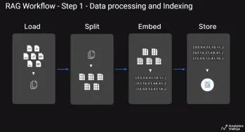
This article explores Retrieval Augmented Generation (RAG) systems and how AI agents can enhance their capabilities. Traditional RAG systems, while useful for leveraging custom enterprise data, suffer from limitations such as a lack of real-time dat


Hot AI Tools

Undresser.AI Undress
AI-powered app for creating realistic nude photos

AI Clothes Remover
Online AI tool for removing clothes from photos.

Undress AI Tool
Undress images for free

Clothoff.io
AI clothes remover

Video Face Swap
Swap faces in any video effortlessly with our completely free AI face swap tool!

Hot Article
Hot Tools

MantisBT
Mantis is an easy-to-deploy web-based defect tracking tool designed to aid in product defect tracking. It requires PHP, MySQL and a web server. Check out our demo and hosting services.

Dreamweaver Mac version
Visual web development tools

SublimeText3 Mac version
God-level code editing software (SublimeText3)

PhpStorm Mac version
The latest (2018.2.1) professional PHP integrated development tool

WebStorm Mac version
Useful JavaScript development tools

