 Technology peripherals
 AI
AI What can training and validation metric graphs tell us in machine learning?
What can training and validation metric graphs tell us in machine learning?
In this article, we will summarize the possible situations of training and verification and introduce what kind of information these charts can provide us.

Let’s start with some simple code. The following code establishes a basic training process framework.
from sklearn.model_selection import train_test_split<br>from sklearn.datasets import make_classification<br>import torch<br>from torch.utils.data import Dataset, DataLoader<br>import torch.optim as torch_optim<br>import torch.nn as nn<br>import torch.nn.functional as F<br>import numpy as np<br>import matplotlib.pyplot as pltclass MyCustomDataset(Dataset):<br>def __init__(self, X, Y, scale=False):<br>self.X = torch.from_numpy(X.astype(np.float32))<br>self.y = torch.from_numpy(Y.astype(np.int64))<br><br>def __len__(self):<br>return len(self.y)<br><br>def __getitem__(self, idx):<br>return self.X[idx], self.y[idx]def get_optimizer(model, lr=0.001, wd=0.0):<br>parameters = filter(lambda p: p.requires_grad, model.parameters())<br>optim = torch_optim.Adam(parameters, lr=lr, weight_decay=wd)<br>return optimdef train_model(model, optim, train_dl, loss_func):<br># Ensure the model is in Training mode<br>model.train()<br>total = 0<br>sum_loss = 0<br>for x, y in train_dl:<br>batch = y.shape[0]<br># Train the model for this batch worth of data<br>logits = model(x)<br># Run the loss function. We will decide what this will be when we call our Training Loop<br>loss = loss_func(logits, y)<br># The next 3 lines do all the PyTorch back propagation goodness<br>optim.zero_grad()<br>loss.backward()<br>optim.step()<br># Keep a running check of our total number of samples in this epoch<br>total += batch<br># And keep a running total of our loss<br>sum_loss += batch*(loss.item())<br>return sum_loss/total<br>def train_loop(model, train_dl, valid_dl, epochs, loss_func, lr=0.1, wd=0):<br>optim = get_optimizer(model, lr=lr, wd=wd)<br>train_loss_list = []<br>val_loss_list = []<br>acc_list = []<br>for i in range(epochs): <br>loss = train_model(model, optim, train_dl, loss_func)<br># After training this epoch, keep a list of progress of <br># the loss of each epoch <br>train_loss_list.append(loss)<br>val, acc = val_loss(model, valid_dl, loss_func)<br># Likewise for the validation loss and accuracy<br>val_loss_list.append(val)<br>acc_list.append(acc)<br>print("training loss: %.5f valid loss: %.5f accuracy: %.5f" % (loss, val, acc))<br><br>return train_loss_list, val_loss_list, acc_list<br>def val_loss(model, valid_dl, loss_func):<br># Put the model into evaluation mode, not training mode<br>model.eval()<br>total = 0<br>sum_loss = 0<br>correct = 0<br>batch_count = 0<br>for x, y in valid_dl:<br>batch_count += 1<br>current_batch_size = y.shape[0]<br>logits = model(x)<br>loss = loss_func(logits, y)<br>sum_loss += current_batch_size*(loss.item())<br>total += current_batch_size<br># All of the code above is the same, in essence, to<br># Training, so see the comments there<br># Find out which of the returned predictions is the loudest<br># of them all, and that's our prediction(s)<br>preds = logits.sigmoid().argmax(1)<br># See if our predictions are right<br>correct += (preds == y).float().mean().item()<br>return sum_loss/total, correct/batch_count<br>def view_results(train_loss_list, val_loss_list, acc_list):<br>plt.rcParams["figure.figsize"] = (15, 5)<br>plt.figure()<br>epochs = np.arange(0, len(train_loss_list)) plt.subplot(1, 2, 1)<br>plt.plot(epochs-0.5, train_loss_list)<br>plt.plot(epochs, val_loss_list)<br>plt.title('model loss')<br>plt.ylabel('loss')<br>plt.xlabel('epoch')<br>plt.legend(['train', 'val', 'acc'], loc = 'upper left')<br><br>plt.subplot(1, 2, 2)<br>plt.plot(acc_list)<br>plt.title('accuracy')<br>plt.ylabel('accuracy')<br>plt.xlabel('epoch')<br>plt.legend(['train', 'val', 'acc'], loc = 'upper left')<br>plt.show()<br><br>def get_data_train_and_show(model, batch_size=128, n_samples=10000, n_classes=2, n_features=30, val_size=0.2, epochs=20, lr=0.1, wd=0, break_it=False):<br># We'll make a fictitious dataset, assuming all relevant<br># EDA / Feature Engineering has been done and this is our <br># resultant data<br>X, y = make_classification(n_samples=n_samples, n_classes=n_classes, n_features=n_features, n_informative=n_features, n_redundant=0, random_state=1972)<br><br>if break_it: # Specifically mess up the data<br>X = np.random.rand(n_samples,n_features)<br>X_train, X_val, y_train, y_val = train_test_split(X, y, test_size=val_size, random_state=1972) train_ds = MyCustomDataset(X_train, y_train)<br>valid_ds = MyCustomDataset(X_val, y_val)<br>train_dl = DataLoader(train_ds, batch_size=batch_size, shuffle=True)<br>valid_dl = DataLoader(valid_ds, batch_size=batch_size, shuffle=True) train_loss_list, val_loss_list, acc_list = train_loop(model, train_dl, valid_dl, epochs=epochs, loss_func=F.cross_entropy, lr=lr, wd=wd)<br>view_results(train_loss_list, val_loss_list, acc_list)
The above code is very simple, it is a basic process of obtaining data, training, and verification. Let’s get to the point.
Scenario 1 - Model seems to learn, but performs poorly in validation or accuracy
Regardless of hyperparameters, model Train loss slowly decreases, but Val loss does not decrease, and Its Accuracy does not indicate that it is learning anything.
For example, in this case, the accuracy of binary classification hovers around 50%.
class Scenario_1_Model_1(nn.Module):<br>def __init__(self, in_features=30, out_features=2):<br>super().__init__()<br>self.lin1 = nn.Linear(in_features, out_features)<br>def forward(self, x):<br>x = self.lin1(x)<br>return x<br>get_data_train_and_show(Scenario_1_Model_1(), lr=0.001, break_it=True)

There is not enough information in the data to allow 'learning', and the training data may not contain enough information to allow the model to 'learn'.
In this case (the training data in the code is random data), this means that it cannot learn anything of substance.
The data must have enough information to learn from. EDA and feature engineering are key! Models learn what can be learned, rather than making up things that don’t exist.
Scenario 2 - Training, validation and accuracy curves are all very unstable
For example, the following code: lr=0.1, bs=128
class Scenario_2_Model_1(nn.Module):<br>def __init__(self, in_features=30, out_features=2):<br>super().__init__()<br>self.lin1 = nn.Linear(in_features, out_features)<br>def forward(self, x):<br>x = self.lin1(x)<br>return x<br>get_data_train_and_show(Scenario_2_Model_1(), lr=0.1)

"Learning rate is too high" or "batch is too small" You can try to reduce the learning rate from 0.1 to 0.001, which means that it will not "bounce", but will decrease smoothly.
get_data_train_and_show(Scenario_1_Model_1(), lr=0.001)

In addition to lowering the learning rate, increasing the batch size will also make it smoother.
get_data_train_and_show(Scenario_1_Model_1(), lr=0.001, batch_size=256)

Scenario 3 - Training loss is close to zero, accuracy looks good, but validation does not go down, and also goes up
class Scenario_3_Model_1(nn.Module):<br>def __init__(self, in_features=30, out_features=2):<br>super().__init__()<br>self.lin1 = nn.Linear(in_features, 50)<br>self.lin2 = nn.Linear(50, 150)<br>self.lin3 = nn.Linear(150, 50)<br>self.lin4 = nn.Linear(50, out_features)<br>def forward(self, x):<br>x = F.relu(self.lin1(x))<br>x = F.relu(self.lin2(x))<br>x = F.relu(self.lin3(x))<br>x = self.lin4(x)<br>return x<br>get_data_train_and_show(Scenario_3_Model_1(), lr=0.001)

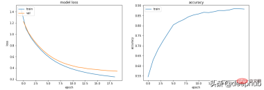
This is definitely overfitting: the training loss is low and the accuracy is high, while the verification loss and training loss are getting larger and larger, which are both classic overfitting indicators.
Fundamentally speaking, your model learning ability is too strong. It remembers the training data too well, which means it also cannot generalize to new data.
The first thing we can try is to reduce the complexity of the model.
class Scenario_3_Model_2(nn.Module):<br>def __init__(self, in_features=30, out_features=2):<br>super().__init__()<br>self.lin1 = nn.Linear(in_features, 50)<br>self.lin2 = nn.Linear(50, out_features)<br>def forward(self, x):<br>x = F.relu(self.lin1(x))<br>x = self.lin2(x)<br>return x<br>get_data_train_and_show(Scenario_3_Model_2(), lr=0.001)

This makes it better, and L2 weight decay regularization can be introduced to make it even better again (for shallower models).
get_data_train_and_show(Scenario_3_Model_2(), lr=0.001, wd=0.02)

If we want to maintain the depth and size of the model, we can try using dropout (for deeper models).
class Scenario_3_Model_3(nn.Module):<br>def __init__(self, in_features=30, out_features=2):<br>super().__init__()<br>self.lin1 = nn.Linear(in_features, 50)<br>self.lin2 = nn.Linear(50, 150)<br>self.lin3 = nn.Linear(150, 50)<br>self.lin4 = nn.Linear(50, out_features)<br>self.drops = nn.Dropout(0.4)<br>def forward(self, x):<br>x = F.relu(self.lin1(x))<br>x = self.drops(x)<br>x = F.relu(self.lin2(x))<br>x = self.drops(x)<br>x = F.relu(self.lin3(x))<br>x = self.drops(x)<br>x = self.lin4(x)<br>return x<br>get_data_train_and_show(Scenario_3_Model_3(), lr=0.001)

场景 4 - 训练和验证表现良好,但准确度没有提高
lr = 0.001,bs = 128(默认,分类类别= 5
class Scenario_4_Model_1(nn.Module):<br>def __init__(self, in_features=30, out_features=2):<br>super().__init__()<br>self.lin1 = nn.Linear(in_features, 2)<br>self.lin2 = nn.Linear(2, out_features)<br>def forward(self, x):<br>x = F.relu(self.lin1(x))<br>x = self.lin2(x)<br>return x<br>get_data_train_and_show(Scenario_4_Model_1(out_features=5), lr=0.001, n_classes=5)

没有足够的学习能力:模型中的其中一层的参数少于模型可能输出中的类。 在这种情况下,当有 5 个可能的输出类时,中间的参数只有 2 个。
这意味着模型会丢失信息,因为它不得不通过一个较小的层来填充它,因此一旦层的参数再次扩大,就很难恢复这些信息。
所以需要记录层的参数永远不要小于模型的输出大小。
class Scenario_4_Model_2(nn.Module):<br>def __init__(self, in_features=30, out_features=2):<br>super().__init__()<br>self.lin1 = nn.Linear(in_features, 50)<br>self.lin2 = nn.Linear(50, out_features)<br>def forward(self, x):<br>x = F.relu(self.lin1(x))<br>x = self.lin2(x)<br>return x<br>get_data_train_and_show(Scenario_4_Model_2(out_features=5), lr=0.001, n_classes=5)

总结
以上就是一些常见的训练、验证时的曲线的示例,希望你在遇到相同情况时可以快速定位并且改进。
The above is the detailed content of What can training and validation metric graphs tell us in machine learning?. For more information, please follow other related articles on the PHP Chinese website!
 Are You At Risk Of AI Agency Decay? Take The Test To Find OutApr 21, 2025 am 11:31 AM
This article explores the growing concern of "AI agency decay"—the gradual decline in our ability to think and decide independently. This is especially crucial for business leaders navigating the increasingly automated world while retainin
 How to Build an AI Agent from Scratch? - Analytics VidhyaApr 21, 2025 am 11:30 AM
Ever wondered how AI agents like Siri and Alexa work? These intelligent systems are becoming more important in our daily lives. This article introduces the ReAct pattern, a method that enhances AI agents by combining reasoning an
 Revisiting The Humanities In The Age Of AIApr 21, 2025 am 11:28 AM
"I think AI tools are changing the learning opportunities for college students. We believe in developing students in core courses, but more and more people also want to get a perspective of computational and statistical thinking," said University of Chicago President Paul Alivisatos in an interview with Deloitte Nitin Mittal at the Davos Forum in January. He believes that people will have to become creators and co-creators of AI, which means that learning and other aspects need to adapt to some major changes. Digital intelligence and critical thinking Professor Alexa Joubin of George Washington University described artificial intelligence as a “heuristic tool” in the humanities and explores how it changes
 Understanding LangChain Agent FrameworkApr 21, 2025 am 11:25 AM
LangChain is a powerful toolkit for building sophisticated AI applications. Its agent architecture is particularly noteworthy, allowing developers to create intelligent systems capable of independent reasoning, decision-making, and action. This expl
 What are the Radial Basis Functions Neural Networks?Apr 21, 2025 am 11:13 AM
Radial Basis Function Neural Networks (RBFNNs): A Comprehensive Guide Radial Basis Function Neural Networks (RBFNNs) are a powerful type of neural network architecture that leverages radial basis functions for activation. Their unique structure make
 The Meshing Of Minds And Machines Has ArrivedApr 21, 2025 am 11:11 AM
Brain-computer interfaces (BCIs) directly link the brain to external devices, translating brain impulses into actions without physical movement. This technology utilizes implanted sensors to capture brain signals, converting them into digital comman
 Insights on spaCy, Prodigy and Generative AI from Ines MontaniApr 21, 2025 am 11:01 AM
This "Leading with Data" episode features Ines Montani, co-founder and CEO of Explosion AI, and co-developer of spaCy and Prodigy. Ines offers expert insights into the evolution of these tools, Explosion's unique business model, and the tr
 A Guide to Building Agentic RAG Systems with LangGraphApr 21, 2025 am 11:00 AM
This article explores Retrieval Augmented Generation (RAG) systems and how AI agents can enhance their capabilities. Traditional RAG systems, while useful for leveraging custom enterprise data, suffer from limitations such as a lack of real-time dat


Hot AI Tools

Undresser.AI Undress
AI-powered app for creating realistic nude photos

AI Clothes Remover
Online AI tool for removing clothes from photos.

Undress AI Tool
Undress images for free

Clothoff.io
AI clothes remover

Video Face Swap
Swap faces in any video effortlessly with our completely free AI face swap tool!

Hot Article

Hot Tools

MantisBT
Mantis is an easy-to-deploy web-based defect tracking tool designed to aid in product defect tracking. It requires PHP, MySQL and a web server. Check out our demo and hosting services.

Dreamweaver Mac version
Visual web development tools

SublimeText3 Mac version
God-level code editing software (SublimeText3)

PhpStorm Mac version
The latest (2018.2.1) professional PHP integrated development tool

WebStorm Mac version
Useful JavaScript development tools


