How to use XGBoost and InluxDB for time series forecasting
XGBoost is a popular open source machine learning library that can be used to solve a variety of prediction problems. One needs to understand how to use it with InfluxDB for time series forecasting.
Translator | Li Rui
Reviewer | Sun Shujuan
XGBoost is an open source machine learning library that implements an optimized distributed gradient boosting algorithm. XGBoost uses parallel processing for fast performance, handles missing values well, performs well on small datasets, and prevents overfitting. All these advantages make XGBoost a popular solution for regression problems such as prediction.
Forecasting is mission-critical for various business goals such as predictive analytics, predictive maintenance, product planning, budgeting, etc. Many forecasting or forecasting problems involve time series data. This makes XGBoost an excellent partner for the open source time series database InfluxDB.
This tutorial will learn how to use XGBoost’s Python package to predict data from the InfluxDB time series database. You will also use the InfluxDB Python client library to query data from InfluxDB and convert the data to a Pandas DataFrame to make it easier to work with time series data before making predictions. Additionally, the advantages of XGBoost will be discussed in more detail.
1. Requirements
This tutorial is performed on a macOS system with Python 3 installed through Homebrew. It is recommended to set up additional tools such as virtualenv, pyenv or conda-env to simplify Python and client installation. Otherwise, its full requirements are as follows:
- influxdb-client=1.30.0
- pandas = 1.4.3
- xgboost>=1.7.3
- influxdb-client>=1.30.0
- pandas>=1.4.3
- matplotlib>=3.5.2
- sklearn>=1.1.1
This tutorial also assumes that you have a free tier InfluxDB cloud account and that you have created a bucket and a token. Think of a bucket as the database or the highest level of data organization in InfluxDB. In this tutorial, a bucket named NOAA will be created.
2. Decision trees, random forests and gradient enhancement
In order to understand what XGBoost is, you must understand decision trees, random forests and gradient enhancement. Decision trees are a supervised learning method consisting of a series of feature tests. Each node is a test, and all nodes are organized in a flowchart structure. Branches represent conditions that ultimately determine which leaf label or class label is assigned to the input data.

# Decision trees in machine learning are used to determine whether it will rain tomorrow. Edited to show the components of a decision tree: leaves, branches, and nodes.
The guiding principle behind decision trees, random forests, and gradient boosting is that multiple "weak learners" or classifiers work together to make strong predictions.
Random forest contains multiple decision trees. Each node in a decision tree is considered a weak learner, and each decision tree in a random forest is considered one of many weak learners in a random forest model. Typically, all data is randomly divided into subsets and passed through different decision trees.
Gradient boosting using decision trees and random forests is similar, but the way they are structured is different. Gradient boosted trees also contain decision tree forests, but these decision trees are additionally constructed and all the data is passed through the decision tree ensemble. Gradient boosting trees may consist of a set of classification trees or regression trees, with classification trees for discrete values (such as cats or dogs). Regression trees are used for continuous values (e.g. 0 to 100).
3. What is XGBoost?
Gradient boosting is a machine learning algorithm used for classification and prediction. XGBoost is just an extreme type of gradient boosting. At its extreme, gradient boosting can be performed more efficiently through the power of parallel processing. The image below from the XGBoost documentation illustrates how gradient boosting can be used to predict whether someone will like a video game.

#Two decision trees are used to decide whether someone is likely to like a video game. Add the leaf scores from both trees to determine which person is most likely to enjoy the video game.
Some advantages of XGBoost:
- Relatively easy to understand.
- Suitable for small, structured and regular data with few features.
Some disadvantages of XGBoost:
- Easy to overfitting and sensitive to outliers. It might be a good idea to use materialized views of time series data in XGBoost for forecasting.
- Performs poorly on sparse or unsupervised data.
4. Use XGBoost for time series prediction
The air sensor sample data set used here is provided by InfluxDB. This dataset contains temperature data from multiple sensors. A temperature forecast is being created for a single sensor with data like this:

Use the following Flux code to import the dataset and filter for a single time series. (Flux is the query language of InfluxDB)
import "join"
import "influxdata/influxdb/sample"
//dataset is regular time series at 10 second intervals
data = sample.data(set: "airSensor")
|> filter(fn: (r) => r._field == "temperature" and r.sensor_id == "TLM0100")
Random forest and gradient boosting can be used for time series forecasting, but they require converting the data to supervised learning. This means that the data must be moved forward in a sliding window approach or a slow-moving approach to convert the time series data into a supervised learning set. The data can also be prepared with Flux. Ideally, some autocorrelation analysis should be performed first to determine the best method to use. For the sake of brevity, the following Flux code will be used to move data at a regular interval.
import "join"
import "influxdata/influxdb/sample"
data = sample.data(set: "airSensor")
|> ; filter(fn: (r) => r._field == "temperature" and r.sensor_id == "TLM0100")
shiftedData = data
|> timeShift(duration : 10s, columns: ["_time"] )
join.time(left: data, right: shiftedData, as: (l, r) => ({l with data: l._value, shiftedData : r._value}))
|> drop(columns: ["_measurement", "_time", "_value", "sensor_id", "_field"])
Swipe left and right to see the complete code

If you want to add additional lag data to the model input, you can follow the following Flux logic instead.
import "experimental"
import "influxdata/influxdb/sample"
data = sample.data(set: "airSensor")
|> ; filter(fn: (r) => r._field == "temperature" and r.sensor_id == "TLM0100")
shiftedData1 = data
|> timeShift(duration: 10s, columns: ["_time"] )
|> set(key: "shift" , value: "1" )
shiftedData2 = data
|> timeShift(duration: 20s , columns: ["_time"] )
|> set(key: "shift" , value: "2" )
shiftedData3 = data
|> timeShift(duration: 30s , columns: ["_time"] )
|> set( key: "shift" , value: "3")
shiftedData4 = data
|> timeShift(duration: 40s , columns: ["_time"] )
|> set(key: "shift" , value: "4")
##union(tables: [shiftedData1, shiftedData2, shiftedData3, shiftedData4])
|> pivot(rowKey:["_time"], columnKey: ["shift"], valueColumn: "_value")
|> drop(columns: ["_measurement", "_time", "_value", "sensor_id", "_field"])
// remove the NaN values
|> limit(n:360)
|> tail(n: 356)

import pandas as pd
from numpy import asarray
from sklearn.metrics import mean_absolute_error
from xgboost import XGBRegressor
from matplotlib import pyplot
from influxdb_client import InfluxDBClient
from influxdb_client.client.write_api import SYNCHRONOUS
# query data with the Python InfluxDB Client Library and transform data into a supervised learning problem with Flux
client = InfluxDBClient(url="https://us-west-2-1.aws.cloud2.influxdata.com", token="NyP-HzFGkObUBI4Wwg6Rbd-_SdrTMtZzbFK921VkMQWp3bv_e9BhpBi6fCBr_0-6i0ev32_XWZcmkDPsearTWA==", org="0437f6d51b579000")
# write_api = client.write_api(write_optinotallow=SYNCHRONOUS)
query_api = client.query_api()
df = query_api.query_data_frame('import "join"'
'import "influxdata/influxdb/sample"'
'data = sample.data(set: "airSensor")'
'|> filter(fn: (r) => r._field == "temperature" and r.sensor_id == "TLM0100")'
'shiftedData = data'
'|> timeShift(duration: 10s , columns: ["_time"] )'
'join.time(left: data, right: shiftedData, as: (l, r) => ({l with data: l._value, shiftedData: r._value}))'
'|> drop(columns: ["_measurement", "_time", "_value", "sensor_id", "_field"])'
'|> yield(name: "converted to supervised learning dataset")'
)
df = df.drop(columns=['table', 'result'])
data = df.to_numpy()
# split a univariate dataset into train/test sets
def train_test_split(data, n_test):
return data[:-n_test:], data[-n_test:]
# fit an xgboost model and make a one step prediction
def xgboost_forecast(train, testX):
# transform list into array
train = asarray(train)
# split into input and output columns
trainX, trainy = train[:, :-1], train[:, -1]
# fit model
model = XGBRegressor(objective='reg:squarederror', n_estimators=1000)
model.fit(trainX, trainy)
# make a one-step prediction
yhat = model.predict(asarray([testX]))
return yhat[0]
# walk-forward validation for univariate data
def walk_forward_validation(data, n_test):
predictions = list()
# split dataset
train, test = train_test_split(data, n_test)
history = [x for x in train]
# step over each time-step in the test set
for i in range(len(test)):
# split test row into input and output columns
testX, testy = test[i, :-1], test[i, -1]
# fit model on history and make a prediction
yhat = xgboost_forecast(history, testX)
# store forecast in list of predictions
predictions.append(yhat)
# add actual observation to history for the next loop
history.append(test[i])
# summarize progress
print('>expected=%.1f, predicted=%.1f' % (testy, yhat))
# estimate prediction error
error = mean_absolute_error(test[:, -1], predictions)
return error, test[:, -1], predictions
# evaluate
mae, y, yhat = walk_forward_validation(data, 100)
print('MAE: %.3f' % mae)
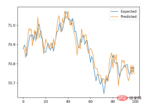
# plot expected vs predicted
pyplot.plot(y, label='Expected')
pyplot.plot(yhat, label='Predicted')
pyplot.legend()
pyplot.show()
五、结论
希望这篇博文能够激励人们利用XGBoost和InfluxDB进行预测。为此建议查看相关的报告,其中包括如何使用本文描述的许多算法和InfluxDB来进行预测和执行异常检测的示例。
原文链接:https://www.infoworld.com/article/3682070/time-series-forecasting-with-xgboost-and-influxdb.html

The above is the detailed content of How to use XGBoost and InluxDB for time series forecasting. For more information, please follow other related articles on the PHP Chinese website!
 Are You At Risk Of AI Agency Decay? Take The Test To Find OutApr 21, 2025 am 11:31 AM
This article explores the growing concern of "AI agency decay"—the gradual decline in our ability to think and decide independently. This is especially crucial for business leaders navigating the increasingly automated world while retainin
 How to Build an AI Agent from Scratch? - Analytics VidhyaApr 21, 2025 am 11:30 AM
Ever wondered how AI agents like Siri and Alexa work? These intelligent systems are becoming more important in our daily lives. This article introduces the ReAct pattern, a method that enhances AI agents by combining reasoning an
 Revisiting The Humanities In The Age Of AIApr 21, 2025 am 11:28 AM
"I think AI tools are changing the learning opportunities for college students. We believe in developing students in core courses, but more and more people also want to get a perspective of computational and statistical thinking," said University of Chicago President Paul Alivisatos in an interview with Deloitte Nitin Mittal at the Davos Forum in January. He believes that people will have to become creators and co-creators of AI, which means that learning and other aspects need to adapt to some major changes. Digital intelligence and critical thinking Professor Alexa Joubin of George Washington University described artificial intelligence as a “heuristic tool” in the humanities and explores how it changes
 Understanding LangChain Agent FrameworkApr 21, 2025 am 11:25 AM
LangChain is a powerful toolkit for building sophisticated AI applications. Its agent architecture is particularly noteworthy, allowing developers to create intelligent systems capable of independent reasoning, decision-making, and action. This expl
 What are the Radial Basis Functions Neural Networks?Apr 21, 2025 am 11:13 AM
Radial Basis Function Neural Networks (RBFNNs): A Comprehensive Guide Radial Basis Function Neural Networks (RBFNNs) are a powerful type of neural network architecture that leverages radial basis functions for activation. Their unique structure make
 The Meshing Of Minds And Machines Has ArrivedApr 21, 2025 am 11:11 AM
Brain-computer interfaces (BCIs) directly link the brain to external devices, translating brain impulses into actions without physical movement. This technology utilizes implanted sensors to capture brain signals, converting them into digital comman
 Insights on spaCy, Prodigy and Generative AI from Ines MontaniApr 21, 2025 am 11:01 AM
This "Leading with Data" episode features Ines Montani, co-founder and CEO of Explosion AI, and co-developer of spaCy and Prodigy. Ines offers expert insights into the evolution of these tools, Explosion's unique business model, and the tr
 A Guide to Building Agentic RAG Systems with LangGraphApr 21, 2025 am 11:00 AM
This article explores Retrieval Augmented Generation (RAG) systems and how AI agents can enhance their capabilities. Traditional RAG systems, while useful for leveraging custom enterprise data, suffer from limitations such as a lack of real-time dat


Hot AI Tools

Undresser.AI Undress
AI-powered app for creating realistic nude photos

AI Clothes Remover
Online AI tool for removing clothes from photos.

Undress AI Tool
Undress images for free

Clothoff.io
AI clothes remover

Video Face Swap
Swap faces in any video effortlessly with our completely free AI face swap tool!

Hot Article

Hot Tools

SecLists
SecLists is the ultimate security tester's companion. It is a collection of various types of lists that are frequently used during security assessments, all in one place. SecLists helps make security testing more efficient and productive by conveniently providing all the lists a security tester might need. List types include usernames, passwords, URLs, fuzzing payloads, sensitive data patterns, web shells, and more. The tester can simply pull this repository onto a new test machine and he will have access to every type of list he needs.

WebStorm Mac version
Useful JavaScript development tools

Atom editor mac version download
The most popular open source editor

EditPlus Chinese cracked version
Small size, syntax highlighting, does not support code prompt function

DVWA
Damn Vulnerable Web App (DVWA) is a PHP/MySQL web application that is very vulnerable. Its main goals are to be an aid for security professionals to test their skills and tools in a legal environment, to help web developers better understand the process of securing web applications, and to help teachers/students teach/learn in a classroom environment Web application security. The goal of DVWA is to practice some of the most common web vulnerabilities through a simple and straightforward interface, with varying degrees of difficulty. Please note that this software


