


Among Excel's functions, there is a function called the magician, which is TEXT. However, today, we prefer to call it a drag queen! why? Please read below!

Just imagine, if functions have careers, what would be the careers of each function? Let’s not talk about anything else. Take TEXT as an example. It can change dates into numbers, numbers into dates, Arabic numerals into uppercase Chinese numerals, and dollar amounts into 10,000 yuan. It can even change the conditional judgment of IF... This is simply A well-deserved drag queen!
Transformation 1: Eight-digit numbers become dates
Many companies use ERP systems, and the date in some systems starts with 8 It is presented in the form of digits. When we export the data in the system, we are likely to see a situation like this:

It is inconvenient to use such dates for data analysis Yes, you need to change it into a standard date format. Please see the performance of TEXT:

Interpretation of the formula:
=TEXT(A2,"00月00日")
A2 is the data that needs to be processed. The secret lies in the "00月00日" part. 0 is a placeholder. symbol, use the year, month and day to divide the 8-digit number into three segments. It should be noted that the division is carried out from right to left. First, the two rightmost digits in column A are regarded as "day", then the next two digits on the left are regarded as "month", and the remaining four digits only need one 0 can represent, these four digits are regarded as "year".
The complete writing method of this formula is: =TEXT(A2,"0000年00月00日"), so that the eight-digit date number can be understood clearly!
Transformation 2: Change the date into eight digits
At some point, you will also encounter the problem of changing the date into eight digits situation, since TEXT can turn an eight-digit number into a date, then of course it is no problem to change it back:

Interpretation of the formula:
=TEXT(H2,"emmdd")
H2 is the data to be processed. The difference is that the following format code is completely different from the last time.
In the first example, the data source we want to process is numbers, so the number placeholder 0 is used. But in this example, the data source is date, so 0 cannot be used. e means "year", which can also be replaced by yyyy, m means "month", and d means "day". One e is four bits, plus two m and two d, it is exactly 8 bits.
Transformation 3: Split date and time
After doing the trick between numbers and dates, let’s see what TEXT is How to split date and time.
This situation is common in attendance data:

#Only by separating the clock-in date and time can we make further statistics. Can TEXT really do that? ?
Split date:

Formula analysis: =TEXT(B2,"e/m/d")
e represents the year, m represents the month, and d represents the day, which is easy to understand.
Split time:

Formula analysis: =TEXT(B2,"h:mm:ss")
#h represents hours, m represents minutes, and s represents seconds.
The trick is revealed and it’s not difficult at all.
But don’t think that you can see through TEXT if you understand these codes. If you don’t believe it, read on...
Transformation Four: Numbers become uppercase Chinese

#How this trick turned out!
Formula analysis: =TEXT(A2,"[DBNUM2]")
DBNUM2 is a specific code for numbers and needs to be placed in a pair of square brackets. The number 2 can also be changed to 1 and 3. You can try it to see the specific effect. Remember to leave a message to tell everyone the results of your test!
By the way, it is also possible to change it to 4. As for 5, 6, 7...
After seeing this example, friends who work in finance will probably have some ideas. Can it be used? What about the TEXT function that turns the amount in the accounting report into an uppercase amount including rounded corners?
You can try it yourself first. If you need any tutorials in this area, remember to leave a message and let us know.
Cross-dressing Five: The amount of Yuan turns into Ten Thousand Yuan
Even the Arabic numerals can be turned into Chinese uppercase numerals, let alone the amount of Yuan turned into Ten thousand Yuan The words are said:

Formula analysis: =TEXT(A2,"0!.00 million yuan")
Same as the first example, 0 is still a placeholder, but there is an extra exclamation mark here. Without the exclamation point, "0.0000" means the number is rounded to four decimal places. In the secret weapon of TEXT, the exclamation point is used to force the addition of characters after the exclamation mark at a certain position in the original content, so the decimal point we see in the cell is actually forcibly added to the left of the thousand digits of the original data, and finally added Adding the suffix "ten thousand yuan" will have this effect.
If you think four decimal places are too many, you can also keep one decimal place:

Formula analysis: =TEXT(A2,"0!.0,10,000 yuan")
In this formula, a comma appears in the middle of the specific code. This comma is actually the thousands separator in the number format:

#After using the thousands separator, the number is reduced by a thousand times, which is equivalent to becoming a thousand yuan Therefore, it only needs to display the decimal point in front of the last digit to turn it into a number in ten thousand yuan.
What! I also want two decimal places...
Although this request is a bit difficult for TEXT, it is not impossible. In the previous example, I had never done anything with the first parameter, I was just playing with the format code. Now it seems that I can’t do it without a trick:

Formula analysis: =TEXT(A2%%,"00,000 yuan")
Add two percent signs after A2 to divide the number in cell A2 Take 10000. Now that the data source has been manipulated, there is no need for an exclamation point in the format code. Just follow the number setting rules. 0.00 means displaying with two decimal places. Of course, you can also use 0.0, 0.000, 0.0000 to set different decimal places.
Transformation 6: Stealing the limelight of IF and making conditional judgments
I played around with dates, times, numbers, and amounts. TEXT, this time it has entered the field of IF again, and even wants to steal the limelight of the IF function:

It seems to be performing well, what kind of trick is this?
Formula analysis: =TEXT((A2-B2)/A2,"Up 0%; Down 0%; Flat;")
This time TEXT does not use the format code, but uses a new prop: the semicolon. After using a semicolon, the TEXT function can make conditional judgments.
The first type, the default judgment:
The routine is TEXT (data, ">0 result; result; = 0 result; text result"). TEXT divides data into four types by default, positive numbers, negative numbers, zero and text. Different types return different results. Each result in the parameter is separated by a semicolon. The value before the first semicolon in the parameter is a positive return value; the value before the second semicolon is a negative return value; the value before the third semicolon is a zero return value, and the last value is text. return value.
When (A2-B2)/A2 is a positive number, it displays the growth rate of increase and percentage; when it is a negative number, it displays the decrease rate and percentage; when it is zero, it displays the same level.
The second type, operator judgment:
In fact, the TEXT function also supports the use of comparison operators as judgment conditions. For example, a score of 85 or more is considered excellent. A score greater than or equal to 60 is considered a passing grade, and a score below 60 is considered a failing grade. The formula using TEXT is as follows: =TEXT(F2,"[>=85]Excellent;[>=60]Qualified;Failed")

In this usage, the condition should be placed within square brackets, followed by the content to be displayed. Finally use a semicolon as a separator between a set of conditions and results.
A TEXT function condition can use up to 3 conditions. If there are more than 3 conditions, the error value #VALUE! will be returned. For some simple judgment problems, using the TEXT function is not only shorter than IF, but also looks more sophisticated.
Isn’t it amazing? If you like this function, please remember to click “Looking”!
Related learning recommendations: excel tutorial
The above is the detailed content of Excel function learning: Drag Queen TEXT()!. For more information, please follow other related articles on the PHP Chinese website!

 MEDIAN formula in Excel - practical examplesApr 11, 2025 pm 12:08 PM
This tutorial explains how to calculate the median of numerical data in Excel using the MEDIAN function. The median, a key measure of central tendency, identifies the middle value in a dataset, offering a more robust representation of central tenden
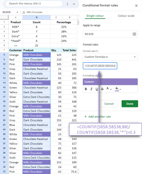 Google Spreadsheet COUNTIF function with formula examplesApr 11, 2025 pm 12:03 PM
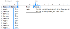
Master Google Sheets COUNTIF: A Comprehensive Guide This guide explores the versatile COUNTIF function in Google Sheets, demonstrating its applications beyond simple cell counting. We'll cover various scenarios, from exact and partial matches to han
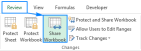 Excel shared workbook: How to share Excel file for multiple usersApr 11, 2025 am 11:58 AM
This tutorial provides a comprehensive guide to sharing Excel workbooks, covering various methods, access control, and conflict resolution. Modern Excel versions (2010, 2013, 2016, and later) simplify collaborative editing, eliminating the need to m
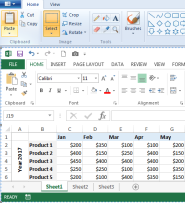 How to convert Excel to JPG - save .xls or .xlsx as image fileApr 11, 2025 am 11:31 AM
This tutorial explores various methods for converting .xls files to .jpg images, encompassing both built-in Windows tools and free online converters. Need to create a presentation, share spreadsheet data securely, or design a document? Converting yo
 Excel names and named ranges: how to define and use in formulasApr 11, 2025 am 11:13 AM
This tutorial clarifies the function of Excel names and demonstrates how to define names for cells, ranges, constants, or formulas. It also covers editing, filtering, and deleting defined names. Excel names, while incredibly useful, are often overlo
 Standard deviation Excel: functions and formula examplesApr 11, 2025 am 11:01 AM
This tutorial clarifies the distinction between standard deviation and standard error of the mean, guiding you on the optimal Excel functions for standard deviation calculations. In descriptive statistics, the mean and standard deviation are intrinsi
 Square root in Excel: SQRT function and other waysApr 11, 2025 am 10:34 AM
This Excel tutorial demonstrates how to calculate square roots and nth roots. Finding the square root is a common mathematical operation, and Excel offers several methods. Methods for Calculating Square Roots in Excel: Using the SQRT Function: The
 Google Sheets basics: Learn how to work with Google SpreadsheetsApr 11, 2025 am 10:23 AM
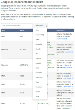
Unlock the Power of Google Sheets: A Beginner's Guide This tutorial introduces the fundamentals of Google Sheets, a powerful and versatile alternative to MS Excel. Learn how to effortlessly manage spreadsheets, leverage key features, and collaborate


Hot AI Tools

Undresser.AI Undress
AI-powered app for creating realistic nude photos

AI Clothes Remover
Online AI tool for removing clothes from photos.

Undress AI Tool
Undress images for free

Clothoff.io
AI clothes remover

Video Face Swap
Swap faces in any video effortlessly with our completely free AI face swap tool!

Hot Article
Hot Tools

VSCode Windows 64-bit Download
A free and powerful IDE editor launched by Microsoft

Atom editor mac version download
The most popular open source editor

EditPlus Chinese cracked version
Small size, syntax highlighting, does not support code prompt function

Dreamweaver CS6
Visual web development tools

SublimeText3 English version
Recommended: Win version, supports code prompts!

