Practical Excel skills sharing: two wonderful ways to find and replace

This article will share with you two wonderful ways to find and replace in Excel. Today you will learn two techniques of summing data by color and identifying qualified data with one click. I hope it will be helpful to you!

Although the two magic tricks shared can be found online, most of them are not as clean and efficient as this tutorial.

Magical Use 1: Sum by color without defining a name

In work, colors are often used to calibrate some data that meet certain conditions. Now that the calibration is done, how to sum by color?

There is some data in the table, some of which are painted in blue and some in gray. Now we need to sum the cell data of the same color:

There are many ways to solve this problem. For example, you can use the macro table function and the sumif function to perform the sum, and you can use the VBA code to perform the sum. Personally, I think using search and replace is a relatively simple method. Let’s take a look at the specific operations:

Operation points:

(1) Use [Select Format from Cell] to absorb colors

(2) After finding all, you need to press Ctrl A to select all and then close the dialog box

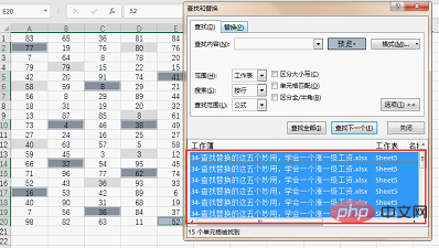
You can use the mouse to click on the result below the search dialog box and then press Ctrl A, and the cells in the table that meet the conditions will be selected.

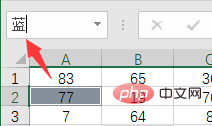
(3) Be sure to press Enter after entering the name box! ! !

# Have you found a place that is more convenient than yours? Or do you have something neater than this?

If you have learned this method, you can try to sum the gray cells yourself.

Magical Use 2: Replace all qualified data with one click without replacement

The previous magical method solved the summation after color marking, and this magical method solves the problem Its previous step: how to identify all qualified data with one click. The logo can be in color or uniformly replaced with certain characters. Let's look at an example of uniform replacement with characters.

As shown in the picture below, it is a student score sheet. When releasing scores, it is required that all scores below 60 are replaced with failing scores without displaying specific scores.

If you were to solve this problem, what would you do except using methods such as functions and custom formats?

The best way to think of is to filter column by column and then replace. In fact, search and replace can be done in one step. Let’s take a look at the operation method:

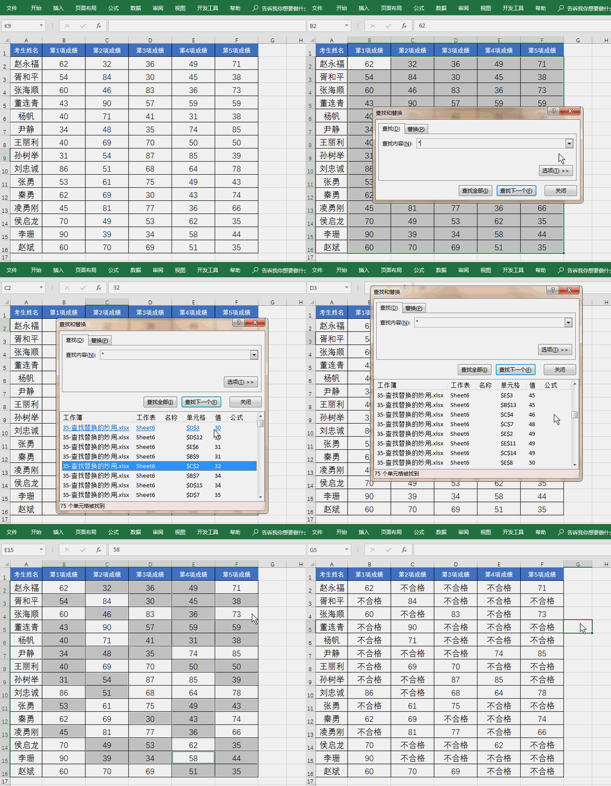
Operation points:

(1) Select the score area first and then search for *;

(2) Click [Value] in the search result Sort;

(3) Select the first result and pull down to find 60. Press the shift key to select the last result above 60, so that the results below can be Cells with 60 points are selected at once;

(4) Do not click the mouse, enter "unqualified" directly, and press the shortcut key Ctrl Enter to complete the operation.

Have you found a place that is more convenient than yours? Or do you have something neater than this?

How about it, are the two tricks I shared today good? Doesn’t it strike you as a complete waste of time?

Related learning recommendations: excel tutorial

The above is the detailed content of Practical Excel skills sharing: two wonderful ways to find and replace. For more information, please follow other related articles on the PHP Chinese website!