Excel function learning lookup function multi-condition matching search application
- 青灯夜游forward
- 2023-01-14 19:03:085275browse
This article shares an Excel formula for calculating sales commission. It mainly uses the lookup function to find matches with multiple conditions. I hope it will be helpful to everyone!

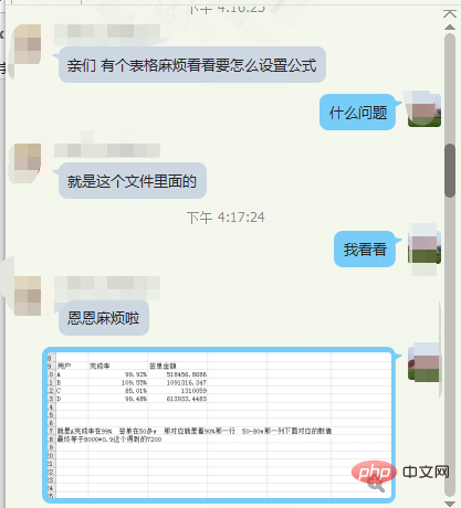
Recently, a student in our learning exchange group raised a question about commission calculation.


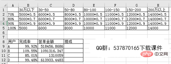
Through simple communication, I roughly understood the student’s problem. As shown in the following table:

#The 1-5 row area is the commission table corresponding to different completion rates and different signing amounts. The area in rows 8-12 is the actual completion rate and order amount of the four users. Now it is necessary to calculate the commission amount of these four users based on the actual completion rate and order amount data.
This example mainly involves the following issues:
1. How to find the corresponding completion rate tier based on the user's completion rate and order amount data?
2. The typesetting method of the commission comparison table is two-dimensional, which makes matching the entire table more difficult.
Let’s analyze and solve this problem step by step with everyone.
Step one: Match the completion rate data to the corresponding gears.
Enter the formula in cell D9:
=LOOKUP(B9,{0.7,0.8,0.9,1})

Analysis:
LOOKUP (find value, search area, return area), the third parameter can be omitted, when omitted the second parameter is as search area and return area.
Note:
The data of the first parameter and the second parameter must be arranged in ascending order, otherwise the function LOOKUP cannot return the correct result, and the text is not case-sensitive.
If the search value is not found in the search area, search for the maximum value in the second parameter that is less than or equal to the search value.
If the lookup value is less than the minimum value in the second parameter, the function LOOKUP returns error value#N/A.
In fact, it can be simply understood as when X finds the value
In this example, the function formula can be understood as X. The completion rate of user A is 0.9992. Through X, we can see that 0.9 is the maximum value less than or equal to 0.9992. Then according to the lookup function search rule, 0.9 should be returned. In this way, we have completed the grading of 4 user completion rates.
Step 2: Complete the grading of the signed amount in the same way.
Enter the formula in cell E9:
=LOOKUP(C9/10000,{0,30,50,80,100,150,200},{"Below 300,000 ","30-50","50-80","80-100","100-150","150-200","More than 2 million"}), double-click to fill in the formula.

Analysis:
In the formula here, LOOKUP has three parameters. The first parameter is the search value, and the second parameter is Search area, the third parameter is to return the specified text.
Step 3: Find the corresponding commission based on the user completion rate and the level of the order amount.
This step is very simple. Find the commission row in the A1-H5 area based on D9, and find the commission column in the A1-H5 area based on E9 to get the corresponding commission result.
Enter the formula in cell F9:
=VLOOKUP(D9,$A$1:$H$5,MATCH(E9,$A$1:$H $1,0),0), double-click to fill.

Analysis:
VLOOKUP (find value, search area, return column, 0)
Match (search value, search area, 0), it should be noted that the search area of the match function can only be a single row and a single column.
The meaning of the formula above: Use the VLOOKUP function to find the row of the D9 cell value in the A1-H5 area, and then use the Match function to find the column of the E9 cell value in the A1-H1 area. , you can get the corresponding commission based on the found row number and column number.
Step 4: Finally, we use the INT function to count the formula calculation results.
First enter ="=INT("&F9&")"


The final result is as follows:

Now the commission data statistics of the number of users have been completed step by step. If you don't want to use the auxiliary column and want to get the result in one step, just combine the above formulas.
In this example, it would be a bit long to combine the function formulas together, but the functions used, except for the LOOKUP function, which requires study, are the most basic and commonly used functions, even if they are Even beginners can easily complete it! In fact, the main purpose of today’s tutorial is to tell you that before you become a master, if you encounter a big problem that is difficult to solve, you can break it into several small problems and solve them one by one. In the end, the big problem will be solved!
Related learning recommendations: excel tutorial
The above is the detailed content of Excel function learning lookup function multi-condition matching search application. For more information, please follow other related articles on the PHP Chinese website!
Related articles
See more- An in-depth analysis of the Excel Tiger Balm screening formula 'INDEX-SMALL-IF-ROW'
- How to quickly export excel return values in Laravel8!
- Practical Excel skills sharing: 5 shortcut keys to improve work efficiency
- Let's talk about five little-known functions of Laravel Excel
- Excel Pivot Table Learning: Three Methods of Dynamically Refreshing Data

