Summarize and sort out several patterned formulas for reverse query in Excel
- WBOYWBOYWBOYWBOYWBOYWBOYWBOYWBOYWBOYWBOYWBOYWBOYWBforward
- 2022-08-19 11:52:442683browse
This article brings you relevant knowledge about excel, which mainly introduces several modular formulas of reverse query. The so-called reverse query means that the keywords are on the right side of the data table. , and the content to be obtained is on the left side of the data table. Let’s take a look at it together. I hope it will be helpful to everyone.

Related learning recommendations: excel tutorial
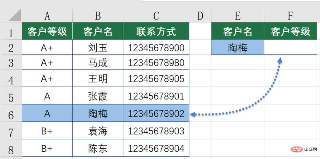
The so-called reverse query means that the keywords are on the right side of the data table, and to get Contents are on the left side of the data sheet.
As shown below, we hope to query the corresponding customer level from the data table on the left based on the customer name specified in cell E2.

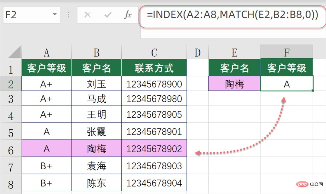
Formula 1:
=INDEX(A2:A8,MATCH(E2,B2:B8,0) )

The patterned usage of this formula is:
=INDEX(area to return content, MATCH(who to look for, search area ,0))
First use the MATCH function to find the position of the query value in a row or column, and then use the INDEX function to return the content of the corresponding position.
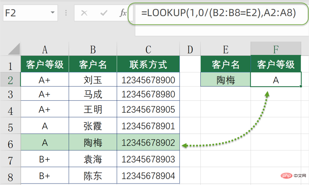
Formula 2:
=LOOKUP(1,0/(B2:B8=E2),A2:A8)

The patterned usage of this formula is:
=LOOKUP(1,0/(lookup area=find content), the area to return the content)
First use the search area of a row or column to compare with the search content one by one to obtain a set of logical values. When the condition is true, the result is TRUE, otherwise it is FALSE.
Then use 0 to divide these logical values, 0 is divided by TRUE, the result is 0, otherwise an error value is returned.
Finally use the LOOKUP function, use 1 as the search value, find the position of 0 in the above memory array, and return the information corresponding to the position in the content area to be returned.
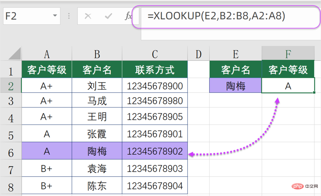
Formula 3:
=XLOOKUP(E2,B2:B8,A2:A8)

The patterned usage of this formula is:
=XLOOKUP (who to look for, where to look for, and what content to return)
The XLOOKUP function is currently available in Excel 2019 and Used in the latest version of WPS forms. Both the search area and the area of returning content need to specify a range of rows and columns.
Related learning recommendations: excel tutorial
The above is the detailed content of Summarize and sort out several patterned formulas for reverse query in Excel. For more information, please follow other related articles on the PHP Chinese website!
Related articles
See more- Sharing practical Excel skills: quickly organize attendance data!
- Learning Excel charts through cases, let's talk about how to draw a graduated cylinder column chart
- 5 ways to use the LOOKUP function in Excel function learning
- Excel function learning: dichotomy principle of LOOKUP function
- Detailed explanation of Excel function COUNTIFS

