


This tutorial explains how to make Excel's VLOOKUP function case sensitive, shows some other formulas that recognize text case, and points out the advantages and limitations of each function.
I think every user using Excel knows what the function in Excel is doing vertical lookup. That's right, it's VLOOKUP. However, few people know that Excel's VLOOKUP is case-insensitive, meaning it treats lowercase and uppercase letters as the same characters.
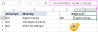
Here is a quick example showing VLOOKUP's ability to be insensitive to text. Suppose you enter "bill" in cell A2 and "Bill" in cell A4. The following formula will capture "bill" because it ranks first in the lookup array and returns the matching value in B2.
=VLOOKUP("Bill", A2:B4, 2, FALSE)

Later in this article, I will show you how to make VLOOKUP case sensitive. We will also explore several other functions that can perform case-sensitive matching in Excel.
Case sensitive VLOOKUP formula ------------------------------------------------------------------------------------------------------------------------------------------------------------------------------------------------------------------------------------------------------As mentioned above, the conventional VLOOKUP formula does not recognize letter case. However, there is a way to make Excel's VLOOKUP case sensitive, as shown in the following example.
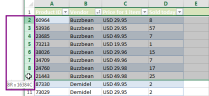
Suppose you enter the item ID in column A and want to pull the price and comments of the item from columns B and C. The problem is that the ID includes upper and lower case characters. For example, the value in A4 (001Tvci3u) and the value in A5 (001Tvci3U) are only different in the last character, namely "u" and "U".
When looking for "001Tvci3 U ", the standard VLOOKUP formula outputs $90 related to "001Tvci3 u " because it is ahead of "001Tvci3 U " in the lookup array. But that's not the result you want, right?
=VLOOKUP(F2, A2:C7, 2, FALSE)

To perform case-sensitive lookups in Excel, we use VLOOKUP, CHOOSE and EXACT functions in combination:
VLOOKUP(TRUE, CHOOSE({1,2}, EXACT( Find value , find array ), return array ), 2, 0) This general formula works perfectly in all cases. You can even look up from right to left, which is something that the regular VLOOKUP formula cannot do. Thanks to Pouriya for coming up with this simple and elegant solution!
In our case, the actual formula is as follows.
To pull the price in F3:
=VLOOKUP(TRUE, CHOOSE({1,2}, EXACT(F2, A2:A7), B2:B7), 2, FALSE)
To get comments in F4:
=VLOOKUP(TRUE, CHOOSE({1,2}, EXACT(F2, A2:A7), C2:C7), 2, FALSE)

Notice. In all versions of Excel except Excel 365, this can only be used as an array formula, so remember to press Ctrl Shift Enter to do it correctly. In Excel 365, it can also be used as a regular formula due to support for dynamic arrays.
How this formula works:
The core part is the CHOOSE formula with EXACT nested:
CHOOSE({1,2}, EXACT(F2, A2:A7), C2:C7)
Here, the EXACT function compares the values in F2 with each in A2:A7 and returns TRUE when they are exactly the same (including letter case), otherwise returns FALSE:
{FALSE;FALSE;FALSE;TRUE;FALSE;FALSE}
For the index_num parameter of CHOOSE, we use the array constant {1,2}. As a result, the function combines the logical values in the above array and the values in C2:C7 into a two-dimensional array, as shown below:
{FALSE,155;FALSE,186;FALSE,90;TRUE,54;FALSE,159;FALSE,28}
The VLOOKUP function takes over from there, looks up the lookup value (i.e. TRUE) in the 2D array (denoted by the logical value) and returns the matching value from the 2nd column, i.e. the price we are looking for:
VLOOKUP(TRUE, {FALSE,155;FALSE,186;FALSE,90;TRUE,54;FALSE,159;FALSE,28}, 2, 0)
Case sensitive XLOOKUP formula
Microsoft 365 subscribers can perform case-sensitive lookups in Excel using simpler formulas. As you can guess, I'm talking about the XLOOKUP function, the stronger successor of VLOOKUP.
Because XLOOKUP operates to find and return arrays separately, we do not need two-dimensional array techniques like the previous example. Simply use EXACT as the search array parameter:
XLOOKUP(TRUE, EXACT( Find value , find array ), return array , "Not Found") The last parameter ("Not Found") is optional. It simply defines the value returned when no match is found. If you omit it, a standard #N/A error will be returned when the formula cannot find a match.
For our sample tables, these are the case sensitive XLOOKUP formulas we use.
To get the price in F3:
=XLOOKUP(TRUE, EXACT(F2, A2:A7), B2:B7, "未找到")
To extract comments in F4:
=XLOOKUP(TRUE, EXACT(F2, A2:A7), C2:C7, "未找到")

How this formula works:
Like the previous example, EXACT returns an array of TRUE and FALSE values, where TRUE represents a case-sensitive match. XLOOKUP looks for the TRUE value in the above array and returns the match from the return array . Note that if there are two or more exactly the same values in the lookup column (including letter case), the formula returns the first found match.
Restrictions of XLOOKUP : Available only in Excel 365 and Excel 2021.
SUMPRODUCT - Case sensitive lookup for returning matching numbers
As the title shows, SUMPRODUCT is another Excel function that can perform case-sensitive lookups, but it can only return numeric values . If this doesn't fit your needs, skip to the INDEX MATCH example, which provides a solution for all data types.
As you probably know, Excel's SUMPRODUCT function multiplies the components in the specified array and returns the sum of the products. Since we want to do case-sensitive searches, we use the EXACT function to get the first array:
=SUMPRODUCT((EXACT(A2:A7,F2) * (B2:B7)))
Unfortunately, the SUMPRODUCT function cannot return a text match because the text values cannot be multiplied. In this case you will get a #VALUE! error in the F4 cell in the screenshot below:

How this formula works:
Like the VLOOKUP example, the EXACT function compares the values in F2 with all values in A2:A7 and returns TRUE on case-sensitive matches, otherwise returns FALSE:
SUMPRODUCT(({FALSE;FALSE;FALSE;TRUE;FALSE;FALSE}*{155;186;90;54;159;28}))
In most formulas, Excel evaluates TRUE to 1 and FALSE to 0. Therefore, when SUMPRODUCT multiplies elements at the same position in two arrays, all non-matches (FALSE) become zero:
SUMPRODUCT({0;0;0;54;0;0})
As a result, the formula returns the number in column B corresponding to the exact case sensitive match in column A.
SUMPRODUCT limit : Only numeric values can be returned.
INDEX MATCH - Case-sensitive lookup for all data types
Finally, we are about to get an unlimited case-sensitive lookup formula that works on all Excel versions and all datasets.
This example is placed at the end not only because the best is left to the end, but also because the knowledge you gained in the previous examples may help you better understand the case-sensitive MATCH INDEX formula.
The combination of INDEX and MATCH functions is often used in Excel as a more flexible and versatile alternative to VLOOKUP. The following article explains how these two functions work together well - using INDEX MATCH instead of VLOOKUP.
Here, I will only remind you some key points:
- The MATCH function searches for the search value in the specified search array and returns its relative position.
- The relative position of the search value is passed directly to the row_num parameter of the INDEX function, guiding it to return a value from the row.
To make the formula recognize text case, you just need to add a function in the classic INDEX MATCH combination. Obviously, you need the EXACT function again:
INDEX ( return array , MATCH(TRUE, EXACT( find value , find array ), 0)) The actual formula in F3 is:
=INDEX(B2:B7, MATCH(TRUE, EXACT(A2:A7, F2), 0))
In F4, we use the following formula:
=INDEX(C2:C7, MATCH(TRUE, EXACT(A2:A7, F2), 0))
Remember that in all versions except Excel 365, it can only be used as an array formula, so make sure to enter it by pressing Ctrl Shift Enter at the same time. If done correctly, the formula will be enclosed in braces, as shown in the screenshot below:

How this formula works:
Like all previous examples, EXACT returns TRUE for each value in A2:A7 that exactly matches the value in F2. Since we use TRUE as the lookup value for MATCH, it returns the relative position of the exact case-sensitive match, which is exactly what INDEX needs to return the match from B2:B7.
Advanced case sensitive search formulas
The INDEX MATCH formula mentioned above looks perfect, right? But in fact, it is not perfect. Let me tell you why.
Assume that the cell corresponding to the search value in the return column is blank. What should the formula return? Return nothing. Now, let's see what it actually returns:
=INDEX(C2:C7, MATCH(TRUE, EXACT(A2:A7, F2), 0))

Oh, the formula returns zero! Maybe this doesn't matter when only text values are processed. However, if your worksheet contains numbers and some of them are real zeros, that's a problem.
In fact, all other search formulas discussed earlier are expressed in the same way. But now you want a perfect formula, don't you?
To make the case-sensitive INDEX MATCH formula absolutely perfect, you can wrap it with an IF function that checks if the return cell is empty and in this case returns a null value:
=IF(INDIRECT("C"&(1 MATCH(TRUE,EXACT(A2:A7, F2), 0)))"", INDEX(C2:C7, MATCH(TRUE, EXACT(A2:A7, F2), 0)), "")
In the above formula:
- "C" is the return column.
- "1" is a number that converts the relative position of the cell returned by the MATCH function into the actual cell address .
For example, the lookup array in our MATCH function is A2:A7, which means that the relative position of cell A2 is "1", because this is the first cell in the array. But in reality, looking for the array starts at line 2. To compensate for the difference, we add 1, so the INDIRECT function will return the value from the correct cell.
The screenshot below shows the actual effect of the improved case-sensitive INDEX MATCH formula.
If the return cell is empty, the formula outputs an empty string:

If the return cell contains zeros, the formula returns 0:

If you would rather show some messages when the return cell is empty, replace the empty string ("") with some text in the last parameter of the IF:
=IF(INDIRECT("C"&(1 MATCH(TRUE, EXACT(A2:A7, F2), 0)))"", INDEX(C2:C7, MATCH(TRUE, EXACT(A2:A7, F2), 0)), "没有可返回的内容,很抱歉。")

Easily perform case-sensitive VLOOKUP
Our users of the Ultimate Excel Suite have a special tool that makes finding in large and complex tables easier and stress-free. The best thing is that the merge two table tools has a case-sensitive option, and the following example shows how it actually works.
Suppose you want to pull Qty from the lookup table based on the unique product ID. into the main table :

All you have to do is run the Merge Table Wizard and perform the following steps:
- Select the main table to pull new data.
- Select a lookup table to find new data.
- Select one or more key columns (in our case the item ID). And make sure to check the case sensitive match box.

- The wizard will walk you through the remaining three steps, where you specify which columns to update, which columns to add, and select some additional options as needed.

After a moment, you will get the desired result :)

This is how to do a lookup that takes into account text case in Excel. Thank you for reading and hope to see you on our blog next week!
Exercise workbook download
Case sensitive VLOOKUP example (.xlsx file)
The above is the detailed content of How to do case-sensitive Vlookup in Excel – formula examples. For more information, please follow other related articles on the PHP Chinese website!

 How to do case-sensitive Vlookup in Excel – formula examplesMay 16, 2025 am 09:42 AM
This tutorial explains how to make Excel's VLOOKUP function case sensitive, shows some other formulas that recognize text case, and points out the advantages and limitations of each function. I think every user using Excel knows what the function in Excel is doing vertical lookup. That's right, it's VLOOKUP. However, few people know that Excel's VLOOKUP is case-insensitive, meaning it treats lowercase and uppercase letters as the same characters. Here is a quick example showing VLOOKUP's ability to be insensitive to text. Suppose you enter "bill" in cell A2 and "Bill" in cell A4.
 Excel INDEX MATCH vs. VLOOKUP - formula examplesMay 16, 2025 am 09:22 AM
This tutorial shows how to use INDEX and MATCH functions in Excel and why it is better than VLOOKUP. In recent articles, we strive to explain the basics of VLOOKUP functions to beginners and provide more complex examples of VLOOKUP formulas for advanced users. Now, I'll try not just to persuade you not to use VLOOKUP, but to at least show an alternative to doing vertical lookups in Excel. "Why do I need this?" you might ask. Because VLOOKUP has many limitations, it may prevent you from getting the desired result in many cases. On the other hand, the INDEX MATCH combination is more flexible and has many excellent features that make it in
 How to delete rows in Excel using shortcuts or VBA macroMay 16, 2025 am 09:03 AM
This article introduces various ways to delete rows based on cell values in Excel. You will find hotkeys and Excel VBA codes in this article. You can delete rows automatically, or use standard lookup options in combination with useful shortcut keys. Excel is an ideal tool for storing frequently changing data. However, updating a table after some changes can take a lot of time. Tasks can be as simple as removing all empty lines in Excel. Alternatively, you may need to find and delete duplicate data. One thing we are sure is that no matter the details are increased or decreased, you are always looking for the best solution to help you save time on your current job. For example, you have a market where different suppliers sell their products. For some reason, one of them
 How to convert number to text in Excel - 4 quick waysMay 15, 2025 am 10:10 AM
This tutorial shows how to convert numbers to text in Excel 2016, 2013, and 2010. Learn how to do this using Excel's TEXT function and use numbers to strings to specify the format. Learn how to change the format of numbers to text using the Format Cell… and Text to Column options. If you use an Excel spreadsheet to store long or short numbers, you may want to convert them to text one day. There may be different reasons to change the number stored as a number to text. Here is why you might need to have Excel treat the entered number as text instead of numbers: Search by part rather than the whole number. For example, you might want to find all numbers containing 50, such as 501
 How to make a dependent (cascading) drop-down list in ExcelMay 15, 2025 am 09:48 AM
We recently delved into the basics of Excel Data Validation, exploring how to set up a straightforward drop-down list using a comma-separated list, cell range, or named range.In today's session, we'll delve deeper into this functionality, focusing on
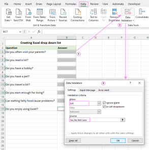 How to create drop down list in Excel: dynamic, editable, searchableMay 15, 2025 am 09:47 AM
This tutorial shows simple steps to create a drop-down list in Excel: Create from cell ranges, named ranges, Excel tables, other worksheets. You will also learn how to make Excel drop-down menus dynamic, editable, and searchable. Microsoft Excel is good at organizing and analyzing complex data. One of its most useful features is the ability to create drop-down menus that allow users to select items from predefined lists. The drop-down menu allows for faster, more accurate and more consistent data entry. This article will show you several different ways to create drop-down menus in Excel. - Excel drop-down list - How to create dropdown list in Excel - From the scope - From the naming range
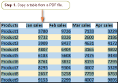 Convert PDF to Excel manually or using online convertersMay 15, 2025 am 09:40 AM
The PDF format, known for its ability to display documents independently of the user's software, hardware, or operating system, has become the standard for electronic file sharing.When requesting information, it's common to receive a well-formatted P
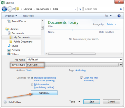 How to convert Excel files to PDFMay 15, 2025 am 09:37 AM
This short tutorial describes 4 possible ways to convert Excel files to PDF - using Excel's Save As feature, Adobe software, online Excel to PDF converter, and desktop tools. Converting an Excel worksheet to a PDF is usually necessary if you want other users to be able to view your data but can't edit it. You may also want to convert Excel spreadsheets to PDF format for use in media toolkits, presentations, and reports, or create a file that all users can open and read even if they don't have Microsoft Excel installed, such as on a tablet or phone. Today, PDF is undoubtedly one of the most popular file formats. According to Google


Hot AI Tools

Undresser.AI Undress
AI-powered app for creating realistic nude photos

AI Clothes Remover
Online AI tool for removing clothes from photos.

Undress AI Tool
Undress images for free

Clothoff.io
AI clothes remover

Video Face Swap
Swap faces in any video effortlessly with our completely free AI face swap tool!

Hot Article
Hot Tools

Zend Studio 13.0.1
Powerful PHP integrated development environment

WebStorm Mac version
Useful JavaScript development tools

SublimeText3 English version
Recommended: Win version, supports code prompts!

SublimeText3 Chinese version
Chinese version, very easy to use

PhpStorm Mac version
The latest (2018.2.1) professional PHP integrated development tool

