


Quick Links
- IF With AND, OR, and NOT
- IFERROR
- IS With IF
Excel's logical functions test whether a statement or data is true or false, before enabling the program to carry out an action based on the result. They are useful for analyzing data, automating certain tasks or calculations, and, ultimately, making decisions.
When used indendently, they return TRUE or FALSE, depending on whether the criteria you set are met.
I'll run through three logical functions (or groups of functions) that I find particularly helpful, and how you can also make the most of them in real-world scenarios.
IF With AND, OR, and NOT
Before I explain how these functions can be used together, I'll explain what each does separately.
AND, OR, and NOT on their own help determine the conditions. In the example below, I want to work out three things for each applicant:
- Are they over 18 and gold-certified (column F)?
- Do they either have a full driving license or the ability to work abroad (column G)?
- Are they not over 50 (column H)?

In cell F2, I need to type
=AND(B2>18,D2="Gold")
because I want Excel to tell me whether the value in B2 is greater than 18 and the value in D2 is equal to "Gold".
In cell G2, I'll type
=AND(B2>18,D2="Gold")
because I want Excel to identify whether the value in C2 is "Full" or the value in E2 is "Yes".
Finally, in cell H2, I'll need to type
=OR(C2="Full",E2="YES")
because I need to check that the value in cell B2 is not greater than 50.
When creating logical arguments, all text needs to go inside double quotes.
Then, I'll use Excel's AutoFill to copy the formulas to the remaining rows.

Notice how each output is either TRUE or FALSE, depending on whether the conditions have been met. While this is handy, having a specific indicator word or phrase can be even more useful. That's where IF comes into play, as it returns a specific value depending on the set conditions.
This time, I want to achieve the following outcomes for each applicant:
- If they are over 18 and gold-certified, they can be labeled as a senior member.
- If they either have a full driving license or the ability to work abroad, they can be labeled as an applicant who can travel.
- If they are not over 50, I want Excel to attach a label that tells me they qualify for an apprenticeship.
So, in cell F2, I'll type
=NOT(B2>50)
because I want Excel to check that the value in B2 is greater than 18 and the value in D2 is "Gold", and then return "Senior" if both are true or "Junior" if not.
In cell G2, I need to go with
=IF(AND(B2>18,D2="Gold"),"Senior","Junior")
because if the value in C2 is "Full" or the value in E2 is "Yes", I need to know that they "Can travel". If neither argument is correct, they "Cannot travel".
Finally, in cell F2, I'll type
=IF(OR(C2="Full",E2="YES"),"Can travel","Cannot travel")
because if the value in B2 is not greater than 50, the applicant is "Eligible for scholarship", but if it is greater than 50, it's "No scholarship".
Again, I will drag the AutoFill handles down for all three columns to populate the remaining rows of my table.

Try using IF, AND, and OR with checkboxes in Excel to track task progress. You can also opt for the XOR function, which, in its simplest form, returns TRUE if only one is TRUE, or FALSE if both values are TRUE.
IFERROR
I use IFERROR to keep all my spreadsheets tidy. After all, nobody wants a spreadsheet full of #N/A, #VALUE!, #REF!, #DIV/0!, #NUM!, #NAME?, and #NULL! errors, and the IFERROR helps to prevent this.
In this example, I am tracking the goals-per-game ratio of ten players. To do this, I typed
=AND(B2>18,D2="Gold")
into cell D2, and then extended this calculation down the whole of column D.
However, because player C has not played any games, the division returns #DIV/0!.

To tidy this up, I would embed all calculations in column D within the IFERROR function.
=OR(C2="Full",E2="YES")
where x is the calculation being performed, and y is the value to return if there is an error.
If you leave y blank after the comma, Excel will return 0 for an erroneous calculation.
So, in cell D2, I will type
=NOT(B2>50)
and extend this down the column. Notice how the
=IF(AND(B2>18,D2="Gold"),"Senior","Junior")
calculation is still there, but it's embedded within the IFERROR function. In this case, anytime there is an error in the calculation, it will return a dash, which looks much tidier than an error message.

Bear in mind that using IFERROR to hide the errors in the spreadsheet can make identifying calculation errors more difficult. This is why I only tend to use it in scenarios when #DIV/0! would otherwise appear.
IS With IF
There are several IS functions, and each of them does very different things. I use them often (within the IF function) to check whether there are any errors or inconsistencies within my data.
Before we look at how to combine them with the IF function, let's look at them in isolation.
All IS functions have the same syntax:
=AND(B2>18,D2="Gold")
where [TYPE] is the type of IS function you want to use, and a is the cell reference or value to be evaluated.
Here are the types of IS functions you can choose from, and you can see some examples below:
- ISBLANK: Tests whether a is blank.
- ISOMITTED: Tests whether the value in a LAMBDA function is missing.
- ISERROR: Tests whether a is an error value (such as #N/A, #VALUE#, and so on).
- ISERR: Tests whether a is any error value except for #N/A.
- ISNA: Tests whether a specifically contains an #N/A error.
- ISFORMULA: Tests whether a is a formula.
- ISLOGICAL: Tests whether a contains a logical value (TRUE or FALSE) based on a logical function.
- ISTEXT: Tests whether a is text, including text produced through a logical function.
- ISNONTEXT: Tests whether a is not text (such as a formula or a number), including text produced through a logical function.
- ISNUMBER: Tests whether a is a number, including a number produced through a formula.
- ISEVEN or ISODD: Tests whether a is an even or an odd number, depending on which one you use. In these cases, a blank cell is seen as even, and a non-numeric cell returns an error.
- ISREF: Tests whether a is a cell reference. For example, if a is (A1), this will return TRUE, but if a is ("apple"), this will return FALSE.
Even though they start with IS, the ISPMT and ISOWEEKNUM functions are not part of the IS group.
Let's look at some of these in an Excel spreadsheet. In columns B to J, I used the specified IS functions to test the values in column A.

For example, in cell B2, I typed
=AND(B2>18,D2="Gold")
and in cell G4, I typed
=OR(C2="Full",E2="YES")
If your IS formula references a cell in a formatted Excel table, the value in the parentheses would be the column name. In the example above, typing
=NOT(B2>50)
into cell F1 would then automatically apply it to the other cells in column F in the table.
To use the IS functions with IF, you need to embed the former inside the latter.
=IF(AND(B2>18,D2="Gold"),"Senior","Junior")
where [TYPE] is the type of IS function you want to use from the list above, a is the cell reference or value to be evaluated, b is the value or formula if TRUE, and c is the value or formula if FALSE.
In the example below, I wanted to work out my employees' projected weekly profits based on their daily profits, but produce a message if the daily profit is blank. To do this, I typed this formula into C2:
=IF(OR(C2="Full",E2="YES"),"Can travel","Cannot travel")
because I wanted Excel to work out whether cell B2 was blank, and either return "Data required" (if B2 was blank) or multiply the value in B2 by seven (if it wasn't blank). I then used AutoFill to copy the relative formula to the remaining cells in column C.

You could do the same with any of the IS functions listed above.
As well as using Excel's logical functions, I use various other combinations of functions to evaluate and use data in Excel's tables, such as INDEX with MATCH, and COUNTIF with SUM. If you're not familiar with these, it's certainly worth giving them a go!
The above is the detailed content of The 3 Best Logical Functions I Always Use in Excel. For more information, please follow other related articles on the PHP Chinese website!

 Excel CONCATENATE function to combine strings, cells, columnsApr 30, 2025 am 10:23 AM
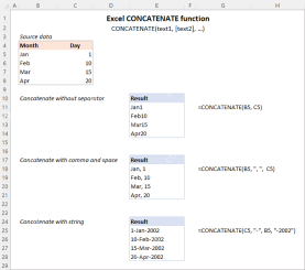
This article explores various methods for combining text strings, numbers, and dates in Excel using the CONCATENATE function and the "&" operator. We'll cover formulas for joining individual cells, columns, and ranges, offering solutio
 Merge and combine cells in Excel without losing dataApr 30, 2025 am 09:43 AM
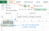
This tutorial explores various methods for efficiently merging cells in Excel, focusing on techniques to retain data when combining cells in Excel 365, 2021, 2019, 2016, 2013, 2010, and earlier versions. Often, Excel users need to consolidate two or
 Excel: Compare two columns for matches and differencesApr 30, 2025 am 09:22 AM
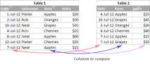
This tutorial explores various methods for comparing two or more columns in Excel to identify matches and differences. We'll cover row-by-row comparisons, comparing multiple columns for row matches, finding matches and differences across lists, high
 Rounding in Excel: ROUND, ROUNDUP, ROUNDDOWN, FLOOR, CEILING functionsApr 30, 2025 am 09:18 AM
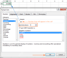
This tutorial explores Excel's rounding functions: ROUND, ROUNDUP, ROUNDDOWN, FLOOR, CEILING, MROUND, and others. It demonstrates how to round decimal numbers to integers or a specific number of decimal places, extract fractional parts, round to the
 Consolidate in Excel: Merge multiple sheets into oneApr 29, 2025 am 10:04 AM
This tutorial explores various methods for combining Excel sheets, catering to different needs: consolidating data, merging sheets via data copying, or merging spreadsheets based on key columns. Many Excel users face the challenge of merging multipl
 Calculate moving average in Excel: formulas and chartsApr 29, 2025 am 09:47 AM
This tutorial shows you how to quickly calculate simple moving averages in Excel, using functions to determine moving averages over the last N days, weeks, months, or years, and how to add a moving average trendline to your charts. Previous articles
 How to calculate average in Excel: formula examplesApr 29, 2025 am 09:38 AM
This tutorial demonstrates various methods for calculating averages in Excel, including formula-based and formula-free approaches, with options for rounding results. Microsoft Excel offers several functions for averaging numerical data, and this gui
 How to calculate weighted average in Excel (SUM and SUMPRODUCT formulas)Apr 29, 2025 am 09:32 AM
This tutorial shows you two simple ways to calculate weighted averages in Excel: using the SUM or SUMPRODUCT function. Previous articles covered basic Excel averaging functions. But what if some values are more important than others, impacting the f


Hot AI Tools

Undresser.AI Undress
AI-powered app for creating realistic nude photos

AI Clothes Remover
Online AI tool for removing clothes from photos.

Undress AI Tool
Undress images for free

Clothoff.io
AI clothes remover

Video Face Swap
Swap faces in any video effortlessly with our completely free AI face swap tool!

Hot Article
Hot Tools

SublimeText3 Chinese version
Chinese version, very easy to use

EditPlus Chinese cracked version
Small size, syntax highlighting, does not support code prompt function

Safe Exam Browser
Safe Exam Browser is a secure browser environment for taking online exams securely. This software turns any computer into a secure workstation. It controls access to any utility and prevents students from using unauthorized resources.

WebStorm Mac version
Useful JavaScript development tools

PhpStorm Mac version
The latest (2018.2.1) professional PHP integrated development tool

