NeRF是什麼？基於NeRF的三維重建是基於體素嗎？

1介紹

神經輻射場（NeRF）是深度學習和電腦視覺領域的一個相當新的範式。 ECCV 2020論文《NeRF：將場景表示為視圖合成的神經輻射場》(該論文獲得了最佳論文獎)中介紹了這項技術，該技術自此大受歡迎，迄今已獲得近800次引用[ 1]。此方法標誌著機器學習處理3D資料的傳統方式發生了巨大變化。

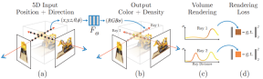
神經輻射場場景表示和可微分渲染過程：

透過沿著相機射線採樣5D座標（位置和觀看方向）來合成影像；將這些位置輸入MLP以產生顏色和體積密度；並使用體積渲染技術將這些值合成影像；此渲染函數是可微分的，因此可以透過最小化合成影像和真實觀測影像之間的殘差來優化場景表示。

2 What is a NeRF?

NeRF是一種生成模型，以圖像和精確姿勢為條件，產生給定圖像的3D場景的新視圖，這一過程通常被稱為為“新視圖合成”。不僅如此，它還將場景的3D形狀和外觀明確定義為連續函數，可以透過marching cubes產生3D網格。儘管它們直接從影像資料中學習，但它們既不使用convolutional層，也不使用transformer層。

多年來，機器學習應用中表示3D資料的方法很多，從3D體素到點雲，再到符號距離(signed distance )函數。他們最大的共同缺點是需要預先假設一個3D模型，要麼使用攝影測量或光達等工具來產生3D數據，要麼手工製作3D模型。然而，許多類型的物體，如高反射物體、「網格狀」物體或透明物體，都無法按比例掃描。 3D重建方法通常也具有重建誤差，這可能導致影響模型精度的階梯效應或漂移。

相較之下，NeRF是基於射線光場的概念。光場是描述光傳輸如何在整個3D體積中發生的函數。它描述了光線在空間中的每個x=(x，y，z）座標和每個方向d上移動的方向，描述為θ和ξ角或單位向量。它們共同形成了描述3D場景中的光傳輸的5D特徵空間。受此表示的啟發，NeRF試圖近似一個函數，該函數從該空間映射到由顏色c=(R，G，B)和濃度(density)σ組成的4D空間，可以將其視為該5D坐標空間處的光線終止的可能性(例如透過遮蔽)。因此，標準NeRF是形式F:（x，d）->（c，σ）的函數。

原始的NeRF論文使用多層感知器將該函數參數化，該感知器基於一組姿勢已知的圖像上訓練得到。這是一類稱為generalized scene reconstruction的技術中的一種方法，旨在直接從圖像集合中描述3D場景。這種方法具備一些非常好的特性：

• 直接從資料中學習
• 場景的連續表示允許非常薄和複雜的結構，例如樹葉或網格
• 隱含物理特性，如鏡面性和粗糙度
• 隱式呈現場景中的照明

此後，一系列的改進論文隨之湧現，例如，少鏡頭與單鏡頭學習[2，3]、對動態場景的支援[4，5]、將光場推廣到特徵場[6]、從網路上的未校準影像集合中學習[7]、結合雷射雷達數據[8]、大規模場景表示[9]、在沒有神經網路的情況下學習[10]，諸如此類。

3 NeRF Architecture

總體而言，給定一個經過訓練的NeRF模型和一個具有已知姿勢和圖像維度的相機，我們透過以下過程建立場景：

• 對於每個像素，從相機光心射出光線穿過場景，以在(x，d)位置收集一組樣本
• 使用每個樣本的點和視線方向(x， d)作為輸入，以產生輸出(c，σ)值(rgbσ)
• 使用經典的體積渲染技術構建圖像

光射場(很多文獻翻譯為"輻射場"，但譯者認為"光射場"更直觀)函數只是幾個組件中的一個，一旦組合起來，就可以創建之前看到的視頻中的視覺效果。整體而言，本文包括以下幾個部分：

• 位置編碼(Positional encoding)
• 光射場函數近似器(MLP）
• 可微分體渲染器(Differentiable volume renderer)
• 分層(Stratified)取樣層次(Hierarchical)體積採樣

為了最大限度地清晰講述，本文將每個組件的關鍵元素以盡可能簡潔的程式碼展示。參考了bmild的原始實現和yenchenlin和krrish94的PyTorch實現。

3.1 Positional Encoder

就像2017年推出的transformer模型[11]一樣，NeRF也受益於位置編碼器作為其輸入。它使用高頻函數將其連續輸入映射到更高維的空間，以幫助模型學習資料中的高頻變化，從而產生更清晰的模型。這種方法避開(circumvent)了神經網路對低頻函數偏置(bias)，使NeRF能夠表示更清晰的細節。作者參考了ICML 2019上的一篇論文[12]。

如果熟悉transformerd的位置編碼，NeRF的相關實作是很標準的，它具有相同的交替正弦和餘弦表達式。位置編碼器實作:

# pyclass PositionalEncoder(nn.Module):# sine-cosine positional encoder for input points.def __init__( self,d_input: int,n_freqs: int,log_space: bool = False ):super().__init__()self.d_input = d_inputself.n_freqs = n_freqs # 是不是视线上的采样频率？self.log_space = log_spaceself.d_output = d_input * (1 + 2 * self.n_freqs)self.embed_fns = [lambda x: x] # 冒号前面的x表示函数参数，后面的表示匿名函数运算# Define frequencies in either linear or log scaleif self.log_space:freq_bands = 2.**torch.linspace(0., self.n_freqs - 1, self.n_freqs)else:freq_bands = torch.linspace(2.**0., 2.**(self.n_freqs - 1), self.n_freqs)# Alternate sin and cosfor freq in freq_bands:self.embed_fns.append(lambda x, freq=freq: torch.sin(x * freq))self.embed_fns.append(lambda x, freq=freq: torch.cos(x * freq))def forward(self, x) -> torch.Tensor:# Apply positional encoding to input.return torch.concat([fn(x) for fn in self.embed_fns], dim=-1)

思考：這個位置編碼，是對輸入點(input points)進行編碼，這個輸入點是視線上的取樣點？還是不同的視角位置點？ self.n_freqs是不是視線上的取樣頻率？由此理解，應該是視線上的採樣位置，因為如果不對視線上的採樣位置進行編碼，就無法有效表示這些位置，也就無法對它們的RGBA進行訓練。

3.2 Radiance Field Function

在原文中，光射場函數由NeRF模型表示，NeRF模型是一種典型的多層感知器，以編碼的3D點和視角方向作為輸入，並傳回RGBA值作為輸出。雖然本文使用的是神經網絡，但這裡可以使用任何函數逼近器(function approximator)。例如，Yu等人的後續論文Plenoxels使用球面諧波(spherical harmonics)實現了數量級的更快訓練，同時獲得有競爭力的結果[10]。

圖片

NeRF模型有8層深，大多數層的特徵維度為256。剩餘的連接被放置在層4處。在這些層之後，產生RGB和σ值。 RGB值以線性層進一步處理，然後與視線方向連接，然後通過另一個線性層，最後在輸出處與σ重新組合。 NeRF模型的PyTorch模組實作：

class NeRF(nn.Module):# Neural radiance fields module.def __init__( self,d_input: int = 3,n_layers: int = 8,d_filter: int = 256,skip: Tuple[int] = (4,), # (4,)只有一个元素4的元组 d_viewdirs: Optional[int] = None): super().__init__()self.d_input = d_input# 这里是3D XYZ,？self.skip = skip# 是要跳过什么？为啥要跳过？被遮挡？self.act = nn.functional.reluself.d_viewdirs = d_viewdirs# d_viewdirs 是2D方向？# Create model layers# [if_true 就执行的指令] if [if_true条件] else [if_false]# 是否skip的区别是，训练输入维度是否多3维，# if i in skip =if i in (4,),似乎是判断i是否等于4# self.d_input=3 ：如果层id=4,网络输入要加3维，这是为什么？第4层有何特殊的？self.layers = nn.ModuleList([nn.Linear(self.d_input, d_filter)] +[nn.Linear(d_filter + self.d_input, d_filter) if i in skip else \ nn.Linear(d_filter, d_filter) for i in range(n_layers - 1)])# Bottleneck layersif self.d_viewdirs is not None:# If using viewdirs, split alpha and RGBself.alpha_out = nn.Linear(d_filter, 1)self.rgb_filters = nn.Linear(d_filter, d_filter)self.branch = nn.Linear(d_filter + self.d_viewdirs, d_filter // 2)self.output = nn.Linear(d_filter // 2, 3) # 为啥要取一半？else:# If no viewdirs, use simpler outputself.output = nn.Linear(d_filter, 4) # d_filter=256，输出是4维RGBAdef forward(self,x: torch.Tensor, # ？viewdirs: Optional[torch.Tensor] = None) -> torch.Tensor: # Forward pass with optional view direction.if self.d_viewdirs is None and viewdirs is not None:raise ValueError('Cannot input x_direction')# Apply forward pass up to bottleneckx_input = x# 这里的x是几维？从下面的分离RGB和A看，应该是4D# 下面通过8层MLP训练RGBAfor i, layer in enumerate(self.layers):# 8层，每一层进行运算x = self.act(layer(x)) if i in self.skip:x = torch.cat([x, x_input], dim=-1)# Apply bottleneckbottleneck 瓶颈是啥？是不是最费算力的模块？if self.d_viewdirs is not None:# 从网络输出分离A,RGB还需要经过更多训练alpha = self.alpha_out(x)# Pass through bottleneck to get RGBx = self.rgb_filters(x) x = torch.concat([x, viewdirs], dim=-1)x = self.act(self.branch(x)) # self.branch shape: (d_filter // 2)x = self.output(x) # self.output shape: (3)# Concatenate alphas to outputx = torch.concat([x, alpha], dim=-1)else:# Simple outputx = self.output(x)return x

思考：這個NERF類別的輸入輸出是什麼？透過這個類發生了啥？從__init__函數參數看出，主要是對神經網路的輸入、層次和維度等進行設置，輸入了5D數據，也就是視點位置和視線方向，輸出的是RGBA。問題，這個輸出的RGBA是一個點的？還是視線上一串的？如果是一串的，沒有看到位置編碼如何確定每個採樣點的RGBA?

也沒看到採樣間隔之類的說明；如果是一個點，那麼這個RGBA是視線上哪個點的？是眼睛看到的視線採樣點集合成後的點RGBA？從NERF類程式碼可以看出，主要是根據視點位置和視線方向進行了多層前饋訓練，輸入5D的視點位置和視線方向，輸出4D的RGBA。

3.3 可微分體渲染器(Differentiable Volume Renderer)

RGBA輸出點位於3D空間中，因此要將它們合成影像，需要應用論文第4節中方程式1-3中描述的體積積分。本質上，沿著每個像素的視線對所有樣本進行加權求和，以獲得該像素的估計顏色值。每個RGB採樣都以其透明度alpha值加權：α值越高，表示採樣區域不透明的可能性越高，因此沿著射線更遠的點更有可能被遮蔽。累積乘積運算確保了這些進一步的點被抑制。

原始NeRF模型輸出的體繪製：

def raw2outputs(raw: torch.Tensor,z_vals: torch.Tensor,rays_d: torch.Tensor,raw_noise_std: float = 0.0,white_bkgd: bool = False) -> Tuple[torch.Tensor, torch.Tensor, torch.Tensor, torch.Tensor]:# 将原始的NeRF输出转为RGB和其他映射# Difference between consecutive elements of `z_vals`. [n_rays, n_samples]dists = z_vals[..., 1:] - z_vals[..., :-1]# ？这里减法的意义是啥？dists = torch.cat([dists, 1e10 * torch.ones_like(dists[..., :1])], dim=-1)# 将每个距离乘以其对应方向光线的范数，以转换为真实世界的距离（考虑非单位方向）dists = dists * torch.norm(rays_d[..., None, :], dim=-1)# 将噪声添加到模型对密度的预测中，用于在训练期间规范网络(防止漂浮物伪影)noise = 0.if raw_noise_std > 0.:noise = torch.randn(raw[..., 3].shape) * raw_noise_std# Predict density of each sample along each ray. Higher values imply# higher likelihood of being absorbed at this point. [n_rays, n_samples]alpha = 1.0 - torch.exp(-nn.functional.relu(raw[..., 3] + noise) * dists)# Compute weight for RGB of each sample along each ray. [n_rays, n_samples]# The higher the alpha, the lower subsequent weights are driven.weights = alpha * cumprod_exclusive(1. - alpha + 1e-10)# Compute weighted RGB map.rgb = torch.sigmoid(raw[..., :3])# [n_rays, n_samples, 3]rgb_map = torch.sum(weights[..., None] * rgb, dim=-2)# [n_rays, 3]# Estimated depth map is predicted distance.depth_map = torch.sum(weights * z_vals, dim=-1)# Disparity map is inverse depth.disp_map = 1. / torch.max(1e-10 * torch.ones_like(depth_map),depth_map / torch.sum(weights, -1))# Sum of weights along each ray. In [0, 1] up to numerical error.acc_map = torch.sum(weights, dim=-1)# To composite onto a white background, use the accumulated alpha map.if white_bkgd:rgb_map = rgb_map + (1. - acc_map[..., None])return rgb_map, depth_map, acc_map, weightsdef cumprod_exclusive(tensor: torch.Tensor) -> torch.Tensor:# (Courtesy of https://github.com/krrish94/nerf-pytorch)# Compute regular cumprod first.cumprod = torch.cumprod(tensor, -1)# "Roll" the elements along dimension 'dim' by 1 element.cumprod = torch.roll(cumprod, 1, -1)# Replace the first element by "1" as this is what tf.cumprod(..., exclusive=True) does.cumprod[..., 0] = 1.return cumprod

問題：這裡的主要功能是啥？輸入了什麼？輸出了什麼？

3.4 Stratified Sampling

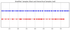
相機最終拾取到的RGB值是沿著穿過該像素視線的光樣本的累積，經典的體積渲染方法是沿著該視線累積點，然後對點進行積分，在每個點估計光線在不撞擊任何粒子的情況下射行的機率。因此，每個像素都需要沿著穿過它的光線對點進行採樣。為了最好地近似積分，他們的分層採樣方法是將空間均勻地劃分為N個倉(bins)，並從每個倉中均勻地抽取一個樣本。 stratified sampling方法不是簡單地以相等的間隔繪製樣本，而是允許模型在連續空間中採樣，從而調節網絡在連續空間上學習。

圖片

分層取樣PyTorch中實作：

def sample_stratified(rays_o: torch.Tensor,rays_d: torch.Tensor,near: float,far: float,n_samples: int,perturb: Optional[bool] = True,inverse_depth: bool = False) -> Tuple[torch.Tensor, torch.Tensor]:# Sample along ray from regularly-spaced bins.# Grab samples for space integration along rayt_vals = torch.linspace(0., 1., n_samples, device=rays_o.device)if not inverse_depth:# Sample linearly between `near` and `far`z_vals = near * (1.-t_vals) + far * (t_vals)else:# Sample linearly in inverse depth (disparity)z_vals = 1./(1./near * (1.-t_vals) + 1./far * (t_vals))# Draw uniform samples from bins along rayif perturb:mids = .5 * (z_vals[1:] + z_vals[:-1])upper = torch.concat([mids, z_vals[-1:]], dim=-1)lower = torch.concat([z_vals[:1], mids], dim=-1)t_rand = torch.rand([n_samples], device=z_vals.device)z_vals = lower + (upper - lower) * t_randz_vals = z_vals.expand(list(rays_o.shape[:-1]) + [n_samples])# Apply scale from `rays_d` and offset from `rays_o` to samples# pts: (width, height, n_samples, 3)pts = rays_o[..., None, :] + rays_d[..., None, :] * z_vals[..., :, None]return pts, z_vals

3.5 層次體積取樣(Hierarchical Volume Sampling)

輻射場由兩個多層感知器表示：一個是在粗略級別上操作，對場景的廣泛結構屬性進行編碼；另一個是在精細的層面上細化細節，從而實現網格和分支等薄而複雜的結構。此外，他們接收的樣本是不同的，粗模型在整個射線中處理寬的、大多是規則間隔的樣本，而精細模型在具有強先驗的區域中珩磨(honing in)以獲得顯著資訊。

这种“珩磨”过程是通过层次体积采样流程完成的。3D空间实际上非常稀疏，存在遮挡，因此大多数点对渲染图像的贡献不大。因此，对具有对积分贡献可能性高的区域进行过采样(oversample)更有好处。他们将学习到的归一化权重应用于第一组样本，以在光线上创建PDF，然后再将inverse transform sampling应用于该PDF以收集第二组样本。该集合与第一集合相结合，并被馈送到精细网络以产生最终输出。

分层采样PyTorch实现：

def sample_hierarchical(rays_o: torch.Tensor,rays_d: torch.Tensor,z_vals: torch.Tensor,weights: torch.Tensor,n_samples: int,perturb: bool = False) -> Tuple[torch.Tensor, torch.Tensor, torch.Tensor]:# Apply hierarchical sampling to the rays.# Draw samples from PDF using z_vals as bins and weights as probabilities.z_vals_mid = .5 * (z_vals[..., 1:] + z_vals[..., :-1])new_z_samples = sample_pdf(z_vals_mid, weights[..., 1:-1], n_samples, perturb=perturb)new_z_samples = new_z_samples.detach()# Resample points from ray based on PDF.z_vals_combined, _ = torch.sort(torch.cat([z_vals, new_z_samples], dim=-1), dim=-1)# [N_rays, N_samples + n_samples, 3]pts = rays_o[..., None, :] + rays_d[..., None, :] * z_vals_combined[..., :, None]return pts, z_vals_combined, new_z_samplesdef sample_pdf(bins: torch.Tensor, weights: torch.Tensor, n_samples: int, perturb: bool = False) -> torch.Tensor:# Apply inverse transform sampling to a weighted set of points.# Normalize weights to get PDF.# [n_rays, weights.shape[-1]]pdf = (weights + 1e-5) / torch.sum(weights + 1e-5, -1, keepdims=True) # Convert PDF to CDF.cdf = torch.cumsum(pdf, dim=-1) # [n_rays, weights.shape[-1]]# [n_rays, weights.shape[-1] + 1]cdf = torch.concat([torch.zeros_like(cdf[..., :1]), cdf], dim=-1) # Take sample positions to grab from CDF. Linear when perturb == 0.if not perturb:u = torch.linspace(0., 1., n_samples, device=cdf.device)u = u.expand(list(cdf.shape[:-1]) + [n_samples]) # [n_rays, n_samples]else:# [n_rays, n_samples]u = torch.rand(list(cdf.shape[:-1]) + [n_samples], device=cdf.device) # Find indices along CDF where values in u would be placed.u = u.contiguous() # Returns contiguous tensor with same values.inds = torch.searchsorted(cdf, u, right=True) # [n_rays, n_samples]# Clamp indices that are out of bounds.below = torch.clamp(inds - 1, min=0)above = torch.clamp(inds, max=cdf.shape[-1] - 1)inds_g = torch.stack([below, above], dim=-1) # [n_rays, n_samples, 2]# Sample from cdf and the corresponding bin centers.matched_shape = list(inds_g.shape[:-1]) + [cdf.shape[-1]]cdf_g = torch.gather(cdf.unsqueeze(-2).expand(matched_shape), dim=-1,index=inds_g)bins_g = torch.gather(bins.unsqueeze(-2).expand(matched_shape), dim=-1, index=inds_g)# Convert samples to ray length.denom = (cdf_g[..., 1] - cdf_g[..., 0])denom = torch.where(denom <h3 id="Training">4 Training</h3><p>论文中训练NeRF推荐的每网络8层、每层256维的架构在训练过程中会消耗大量内存。缓解这种情况的方法是将前传(forward pass)分成更小的部分，然后在这些部分上积累梯度。注意与minibatching的区别：梯度是在采样光线的单个小批次上累积的，这些光线可能已经被收集成块。如果没有论文中使用的NVIDIA V100类似性能的GPU，可能必须相应地调整块大小以避免OOM错误。Colab笔记本采用了更小的架构和更适中的分块尺寸。</p><p>我个人发现，由于局部极小值，即使选择了许多默认值，NeRF的训练也有些棘手。一些有帮助的技术包括早期训练迭代和早期重新启动期间的中心裁剪(center cropping)。随意尝试不同的超参数和技术，以进一步提高训练收敛性。</p><h4 id="初始化">初始化</h4><pre class="brush:php;toolbar:false">def init_models():# Initialize models, encoders, and optimizer for NeRF training.encoder = PositionalEncoder(d_input, n_freqs, log_space=log_space)encode = lambda x: encoder(x)# View direction encodersif use_viewdirs:encoder_viewdirs = PositionalEncoder(d_input, n_freqs_views,log_space=log_space)encode_viewdirs= lambda x: encoder_viewdirs(x)d_viewdirs = encoder_viewdirs.d_outputelse:encode_viewdirs = Noned_viewdirs = Nonemodel = NeRF(encoder.d_output,  n_layers=n_layers,  d_filter=d_filter, skip=skip,d_viewdirs=d_viewdirs)model.to(device)model_params = list(model.parameters())if use_fine_model:fine_model = NeRF(encoder.d_output, n_layers=n_layers, d_filter=d_filter, skip=skip,d_viewdirs=d_viewdirs)fine_model.to(device)model_params = model_params + list(fine_model.parameters())else:fine_model = Noneoptimizer= torch.optim.Adam(model_params, lr=lr)warmup_stopper = EarlyStopping(patience=50)return model, fine_model, encode, encode_viewdirs, optimizer, warmup_stopper

训练

def train():# Launch training session for NeRF.# Shuffle rays across all images.if not one_image_per_step:height, width = images.shape[1:3]all_rays = torch.stack([torch.stack(get_rays(height, width, focal, p), 0) for p in poses[:n_training]], 0)rays_rgb = torch.cat([all_rays, images[:, None]], 1)rays_rgb = torch.permute(rays_rgb, [0, 2, 3, 1, 4])rays_rgb = rays_rgb.reshape([-1, 3, 3])rays_rgb = rays_rgb.type(torch.float32)rays_rgb = rays_rgb[torch.randperm(rays_rgb.shape[0])]i_batch = 0train_psnrs = []val_psnrs = []iternums = []for i in trange(n_iters):model.train()if one_image_per_step:# Randomly pick an image as the target.target_img_idx = np.random.randint(images.shape[0])target_img = images[target_img_idx].to(device)if center_crop and i = rays_rgb.shape[0]:rays_rgb = rays_rgb[torch.randperm(rays_rgb.shape[0])]i_batch = 0target_img = target_img.reshape([-1, 3])# Run one iteration of TinyNeRF and get the rendered RGB image.outputs = nerf_forward(rays_o, rays_d, near, far, encode, model, kwargs_sample_stratified=kwargs_sample_stratified, n_samples_hierarchical=n_samples_hierarchical, kwargs_sample_hierarchical=kwargs_sample_hierarchical, fine_model=fine_model, viewdirs_encoding_fn=encode_viewdirs, chunksize=chunksize)# Backprop!rgb_predicted = outputs['rgb_map']loss = torch.nn.functional.mse_loss(rgb_predicted, target_img)loss.backward()optimizer.step()optimizer.zero_grad()psnr = -10. * torch.log10(loss)train_psnrs.append(psnr.item())# Evaluate testimg at given display rate.if i % display_rate == 0:model.eval()height, width = testimg.shape[:2]rays_o, rays_d = get_rays(height, width, focal, testpose)rays_o = rays_o.reshape([-1, 3])rays_d = rays_d.reshape([-1, 3])outputs = nerf_forward(rays_o, rays_d, near, far, encode, model, kwargs_sample_stratified=kwargs_sample_stratified, n_samples_hierarchical=n_samples_hierarchical, kwargs_sample_hierarchical=kwargs_sample_hierarchical, fine_model=fine_model, viewdirs_encoding_fn=encode_viewdirs, chunksize=chunksize)rgb_predicted = outputs['rgb_map']loss = torch.nn.functional.mse_loss(rgb_predicted, testimg.reshape(-1, 3))val_psnr = -10. * torch.log10(loss)val_psnrs.append(val_psnr.item())iternums.append(i)# Check PSNR for issues and stop if any are found.if i == warmup_iters - 1:if val_psnr <h4 id="训练">训练</h4><pre class="brush:php;toolbar:false"># Run training session(s)for _ in range(n_restarts):model, fine_model, encode, encode_viewdirs, optimizer, warmup_stopper = init_models()success, train_psnrs, val_psnrs = train()if success and val_psnrs[-1] >= warmup_min_fitness:print('Training successful!')breakprint(f'Done!')

5 Conclusion

辐射场标志着处理3D数据的方式发生了巨大变化。NeRF模型和更广泛的可微分渲染正在迅速弥合图像创建和体积场景创建之间的差距。虽然我们的组件可能看起来非常复杂，但受vanilla NeRF启发的无数其他方法证明，基本概念(连续函数逼近器+可微分渲染器)是构建各种解决方案的坚实基础，这些解决方案可用于几乎无限的情况。

原文：NeRF From Nothing: A Tutorial with PyTorch | Towards Data Science

原文链接：https://mp.weixin.qq.com/s/zxJAIpAmLgsIuTsPqQqOVg

以上是NeRF是什麼？基於NeRF的三維重建是基於體素嗎？的詳細內容。更多資訊請關注PHP中文網其他相關文章！