邏輯迴歸，分類：監督機器學習

什麼是分類？

定義和目的

分類是機器學習和資料科學中使用的一種監督學習技術，用於將資料分類為預先定義的類別或標籤。它涉及訓練一個模型，根據輸入資料點的特徵將其分配給幾個離散類別之一。分類的主要目的是準確預測新的、未見過的資料點的類別。

主要目標：

• 預測：將新資料點分配給預先定義的類別之一。
• 估計：確定資料點屬於特定類別的機率。
• 理解關係：辨識哪些特徵對於預測資料點的類別很重要。

分類類型

1。二元分類

• 描述：將資料分類為兩個類別之一。
  • 範例：垃圾郵件偵測（垃圾郵件或非垃圾郵件）、疾病診斷（有病或無疾病）。
  • 目的：區分兩個不同的類別。

2。多類分類

• 描述：將資料分類為三個或更多類別之一。
  • 範例：手寫數字辨識（數字0-9）、花種類分類（多種）。
  • 目的：處理需要預測兩個以上類別的問題。

什麼是線性分類器？

線性分類器是一類分類演算法，它使用線性決策邊界來分離特徵空間中的不同類別。他們透過線性方程式組合輸入特徵來進行預測，通常表示特徵和目標類標籤之間的關係。線性分類器的主要目的是透過找到將特徵空間劃分為不同類別的超平面來有效地將資料點分類。

邏輯迴歸

定義和目的

邏輯迴歸是一種用於機器學習和資料科學中二元分類任務的統計方法。它是線性分類器的一部分，與線性迴歸不同，它透過將資料擬合到邏輯曲線來預測事件發生的機率。

主要目標：

• 二元分類：預測二元結果（例如，是/否、真/假）。
• 機率估計：根據輸入變數估計事件發生的機率。
• 決策邊界：決定將資料分類為不同類別的閾值。

邏輯迴歸模型

1。 Logistic 函數（S 型函數）

• 描述：邏輯函數將任何實值輸入轉換為 0 到 1 之間的值，使其適合機率建模。
  • 方程式: σ(z) = 1 / (1 + e^(-z))
  • 目的：將輸入值對應到機率。

2。邏輯迴歸方程式

• 描述：邏輯迴歸模型將邏輯函數應用於輸入變數的線性組合。
  • 方程式：P(y=1|x) = σ(w0 + w1x1 + w2x2 + ... + wnxn)
  • 目的：在給定輸入變數x的情況下預測二元結果y=1的機率P(y=1|x)。

最大似然估計（MLE）

MLE 用於透過最大化觀察給定模型的資料的可能性來估計邏輯迴歸模型的參數（係數）。

方程式：最大化對數似然函數涉及找到最大化觀察資料的機率的參數。

邏輯迴歸中的成本函數和損失最小化

成本函數

邏輯迴歸中的成本函數衡量預測機率與實際類別標籤之間的差異。目標是最小化此函數以提高模型的預測準確性。

對數損失（二元交叉熵）:
對數損失函數常用於二元分類任務的邏輯迴歸。

對數損失 = -(1/n) * Σ [y * log(ŷ) + (1 - y) * log(1 - ŷ)]

地點：

• y 是實際的類別標籤（0 或 1），
• ŷ 是類別標籤的預測機率，
• n 是資料點的數量。

對數損失會懲罰遠離實際類別標籤的預測，從而鼓勵模型產生準確的機率。

損失最小化（優化）

邏輯迴歸中的

損失最小化涉及找到最小化成本函數值的模型參數值。此過程也稱為最佳化。邏輯迴歸中損失最小化最常用的方法是梯度下降演算法。

梯度下降

梯度下降是一種迭代最佳化演算法，用於最小化邏輯迴歸中的成本函數。它沿著成本函數最速下降的方向調整模型參數。

梯度下降的步驟:

1. 初始化參數：從模型參數的初始值開始（例如係數 w0、w1、...、wn）。

2. 計算梯度：計算成本函數相對於每個參數的梯度。梯度是成本函數的偏導數。

3. 更新參數：向漸變的反方向調整參數。調整由學習率 (α) 控制，它決定了向最小值邁出的步長。

4. 重複：迭代這個過程，直到成本函數收斂到最小值（或達到預先定義的迭代次數）。

參數更新規則:
對於每個參數 wj：
wj = wj - α * (∂/∂wj) 對數損失

地點：

• α 是學習率，
• (∂/∂wj) Log Loss 是對數損失關於 wj 的偏導數。

對數損失關於 wj 的偏導數可以計算為：
(∂/∂wj) 對數損失 = -(1/n) * Σ [ (yi - ŷi) * xij / (ŷi * (1 - ŷi)) ]

地點：

• xij 是第 i 個資料點的第 j 個自變數的值，
• ŷi 是第 i 個資料點的類別標籤的預測機率。

Logistic 迴歸（二元分類）範例

邏輯迴歸是一種用於二元分類任務的技術，對給定輸​​入屬於特定類別的機率進行建模。此範例示範如何使用合成資料實現邏輯迴歸、評估模型的效能以及視覺化決策邊界。

Python 程式碼範例

1。導入庫

import numpy as np
import matplotlib.pyplot as plt
from sklearn.model_selection import train_test_split
from sklearn.linear_model import LogisticRegression
from sklearn.metrics import accuracy_score, confusion_matrix, classification_report

此區塊導入資料操作、繪圖和機器學習所需的庫。

2。產生樣本資料

np.random.seed(42)  # For reproducibility
X = np.random.randn(1000, 2)
y = (X[:, 0] + X[:, 1] > 0).astype(int)

此區塊產生具有兩個特徵的樣本數據，其中根據特徵總和是否大於零來定義目標變數 y，模擬二元分類場景。

3。分割資料集

X_train, X_test, y_train, y_test = train_test_split(X, y, test_size=0.2, random_state=42)

此區塊將資料集拆分為訓練集和測試集以進行模型評估。

4。建立並訓練邏輯迴歸模型

model = LogisticRegression(random_state=42)
model.fit(X_train, y_train)

此區塊初始化邏輯迴歸模型並使用訓練資料集進行訓練。

5。做出預測

y_pred = model.predict(X_test)

此區塊使用經過訓練的模型對測試集進行預測。

6。評估模型

accuracy = accuracy_score(y_test, y_pred)
conf_matrix = confusion_matrix(y_test, y_pred)
class_report = classification_report(y_test, y_pred)

print(f"Accuracy: {accuracy:.4f}")
print("\nConfusion Matrix:")
print(conf_matrix)
print("\nClassification Report:")
print(class_report)

輸出：

Accuracy: 0.9950

Confusion Matrix:
[[ 92   0]
 [  1 107]]

Classification Report:
              precision    recall  f1-score   support

           0       0.99      1.00      0.99        92
           1       1.00      0.99      1.00       108

    accuracy                           0.99       200
   macro avg       0.99      1.00      0.99       200
weighted avg       1.00      0.99      1.00       200

此區塊計算並列印準確性、混淆矩陣和分類報告，提供對模型效能的深入了解。

7。可視化決策邊界

x_min, x_max = X[:, 0].min() - 1, X[:, 0].max() + 1
y_min, y_max = X[:, 1].min() - 1, X[:, 1].max() + 1
xx, yy = np.meshgrid(np.arange(x_min, x_max, 0.1),
                     np.arange(y_min, y_max, 0.1))
Z = model.predict(np.c_[xx.ravel(), yy.ravel()])
Z = Z.reshape(xx.shape)

plt.figure(figsize=(10, 8))
plt.contourf(xx, yy, Z, alpha=0.4)
plt.scatter(X[:, 0], X[:, 1], c=y, alpha=0.8)
plt.xlabel("Feature 1")
plt.ylabel("Feature 2")
plt.title("Logistic Regression Decision Boundary")
plt.show()

此區塊視覺化邏輯迴歸模型所建立的決策邊界，說明模型如何在特徵空間中分離兩個類別。

輸出：

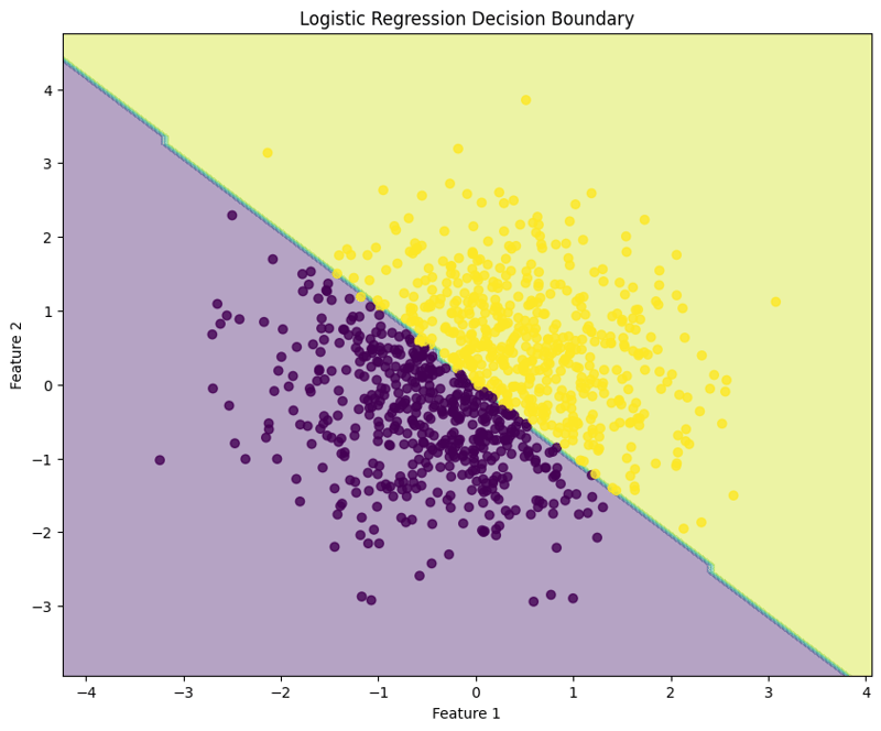
這種結構化方法展示瞭如何實現和評估邏輯回歸，讓人們清楚地了解其二元分類任務的功能。決策邊界的可視化有助於解釋模型的預測。

Logistic Regression (Multiclass Classification) Example

Logistic regression can also be applied to multiclass classification tasks. This example demonstrates how to implement logistic regression using synthetic data, evaluate the model's performance, and visualize the decision boundary for three classes.

Python Code Example

1. Import Libraries

import numpy as np
import matplotlib.pyplot as plt
from sklearn.model_selection import train_test_split
from sklearn.linear_model import LogisticRegression
from sklearn.metrics import accuracy_score, confusion_matrix, classification_report

This block imports the necessary libraries for data manipulation, plotting, and machine learning.

2. Generate Sample Data with 3 Classes

np.random.seed(42)  # For reproducibility
n_samples = 999  # Total number of samples
n_samples_per_class = 333  # Ensure this is exactly n_samples // 3

# Class 0: Top-left corner
X0 = np.random.randn(n_samples_per_class, 2) * 0.5 + [-2, 2]

# Class 1: Top-right corner
X1 = np.random.randn(n_samples_per_class, 2) * 0.5 + [2, 2]

# Class 2: Bottom center
X2 = np.random.randn(n_samples_per_class, 2) * 0.5 + [0, -2]

# Combine the data
X = np.vstack([X0, X1, X2])
y = np.hstack([np.zeros(n_samples_per_class), 
               np.ones(n_samples_per_class), 
               np.full(n_samples_per_class, 2)])

# Shuffle the dataset
shuffle_idx = np.random.permutation(n_samples)
X, y = X[shuffle_idx], y[shuffle_idx]

This block generates synthetic data for three classes located in different regions of the feature space.

3. Split the Dataset

X_train, X_test, y_train, y_test = train_test_split(X, y, test_size=0.2, random_state=42)

This block splits the dataset into training and testing sets for model evaluation.

4. Create and Train the Logistic Regression Model

model = LogisticRegression(random_state=42)
model.fit(X_train, y_train)

This block initializes the logistic regression model and trains it using the training dataset.

5. Make Predictions

y_pred = model.predict(X_test)

This block uses the trained model to make predictions on the test set.

6. Evaluate the Model

accuracy = accuracy_score(y_test, y_pred)
conf_matrix = confusion_matrix(y_test, y_pred)
class_report = classification_report(y_test, y_pred)

print(f"Accuracy: {accuracy:.4f}")
print("\nConfusion Matrix:")
print(conf_matrix)
print("\nClassification Report:")
print(class_report)

Output:

Accuracy: 1.0000

Confusion Matrix:
[[54  0  0]
 [ 0 65  0]
 [ 0  0 81]]

Classification Report:
              precision    recall  f1-score   support

         0.0       1.00      1.00      1.00        54
         1.0       1.00      1.00      1.00        65
         2.0       1.00      1.00      1.00        81

    accuracy                           1.00       200
   macro avg       1.00      1.00      1.00       200
weighted avg       1.00      1.00      1.00       200

This block calculates and prints the accuracy, confusion matrix, and classification report, providing insights into the model's performance.

7. Visualize the Decision Boundary

x_min, x_max = X[:, 0].min() - 1, X[:, 0].max() + 1
y_min, y_max = X[:, 1].min() - 1, X[:, 1].max() + 1
xx, yy = np.meshgrid(np.arange(x_min, x_max, 0.1),
                     np.arange(y_min, y_max, 0.1))
Z = model.predict(np.c_[xx.ravel(), yy.ravel()])
Z = Z.reshape(xx.shape)

plt.figure(figsize=(10, 8))
plt.contourf(xx, yy, Z, alpha=0.4, cmap='RdYlBu')
scatter = plt.scatter(X[:, 0], X[:, 1], c=y, cmap='RdYlBu', edgecolor='black')
plt.xlabel("Feature 1")
plt.ylabel("Feature 2")
plt.title("Multiclass Logistic Regression Decision Boundary")
plt.colorbar(scatter)
plt.show()

This block visualizes the decision boundaries created by the logistic regression model, illustrating how the model separates the three classes in the feature space.

Output:

This structured approach demonstrates how to implement and evaluate logistic regression for multiclass classification tasks, providing a clear understanding of its capabilities and the effectiveness of visualizing decision boundaries.

Evaluating Logistic Regression Model

Evaluating a logistic regression model involves assessing its performance in predicting binary or multiclass outcomes. Below are key methods for evaluation:

1. Performance Metrics

• Accuracy: The proportion of correctly classified instances out of the total instances. It provides a general sense of the model's performance.
  • Formula: Accuracy = (TP + TN) / (TP + TN + FP + FN)

  from sklearn.metrics import accuracy_score

  accuracy = accuracy_score(y_test, y_pred)
  print(f'Accuracy: {accuracy:.4f}')

• Confusion Matrix: A table that summarizes the performance of the classification model by showing the true positives (TP), true negatives (TN), false positives (FP), and false negatives (FN).

  from sklearn.metrics import confusion_matrix

  conf_matrix = confusion_matrix(y_test, y_pred)
  print("\nConfusion Matrix:")
  print(conf_matrix)

• Precision: Measures the accuracy of the positive predictions. It is the ratio of true positives to the sum of true and false positives.
  • Formula: Precision = TP / (TP + FP)

  from sklearn.metrics import precision_score

  precision = precision_score(y_test, y_pred, average='weighted')
  print(f'Precision: {precision:.4f}')

• Recall (Sensitivity): Measures the model's ability to identify all relevant instances (true positives). It is the ratio of true positives to the sum of true positives and false negatives.
  • Formula: Recall = TP / (TP + FN)

  from sklearn.metrics import recall_score

  recall = recall_score(y_test, y_pred, average='weighted')
  print(f'Recall: {recall:.4f}')

• F1 Score: The harmonic mean of precision and recall, providing a balance between the two metrics. It is useful when the class distribution is imbalanced.
  • Formula: F1 Score = 2 * (Precision * Recall) / (Precision + Recall)

  from sklearn.metrics import f1_score

  f1 = f1_score(y_test, y_pred, average='weighted')
  print(f'F1 Score: {f1:.4f}')

2. Cross-Validation

Cross-validation techniques provide a more reliable evaluation of model performance by assessing it across different subsets of the dataset.

• K-Fold Cross-Validation: The dataset is divided into k subsets, and the model is trained on k-1 subsets while validating on the remaining subset. This is repeated k times, and the average metric provides a robust evaluation.

  from sklearn.model_selection import KFold, cross_val_score

  kf = KFold(n_splits=5, shuffle=True, random_state=42)
  scores = cross_val_score(model, X, y, cv=kf, scoring='accuracy')
  print(f'Cross-Validation Accuracy: {np.mean(scores):.4f}')

• Stratified K-Fold Cross-Validation: Similar to K-Fold but ensures that each fold maintains the class distribution, which is particularly beneficial for imbalanced datasets.

  from sklearn.model_selection import StratifiedKFold

  skf = StratifiedKFold(n_splits=5)
  scores = cross_val_score(model, X, y, cv=skf, scoring='accuracy')
  print(f'Stratified K-Fold Cross-Validation Accuracy: {np.mean(scores):.4f}')

By utilizing these evaluation methods and cross-validation techniques, practitioners can gain insights into the effectiveness of their logistic regression model and its ability to generalize to unseen data.

Regularization in Logistic Regression

Regularization helps mitigate overfitting in logistic regression by adding a penalty term to the loss function, encouraging simpler models. The two primary forms of regularization in logistic regression are L1 regularization (Lasso) and L2 regularization (Ridge).

L2 正規化（嶺 Logistic 迴歸）

概念：L2正則化在損失函數中加入等於係數大小平方的懲罰。

損失函數：嶺邏輯迴歸的修正損失函數表示為：

損失 = -Σ[yi * log(ŷi) + (1 - yi) * log(1 - ŷi)] + λ * Σ(wj^2)

地點：

• yi 是實際的類別標籤。
• ŷi 是正類的預測機率。
• wj 是模型係數。
• λ 是正規化參數。

效果：

• 嶺正則化將係數縮小到零，但並沒有消除它們。所有特徵都保留在模型中，這對於具有許多預測變數或多重共線性的情況是有益的。

L1 正規化（Lasso Logistic 迴歸）

概念：L1正則化在損失函數中加入等於係數振幅絕對值的懲罰。

損失函數：Lasso邏輯迴歸的修改損失函數可以表示為：

損失 = -Σ[yi * log(ŷi) + (1 - yi) * log(1 - ŷi)] + λ * Σ|wj|

地點：

• yi 是實際的類別標籤。
• ŷi 是正類的預測機率。
• wj 是模型係數。
• λ 是正規化參數。

效果：

• Lasso 正規化可以將一些係數設為零，從而有效地執行變數選擇。這在可解釋性至關重要的高維資料集中是有利的。

透過在邏輯迴歸中應用正規化技術，從業者可以增強模型泛化並有效管理偏差-變異數權衡。

以上是邏輯迴歸，分類：監督機器學習的詳細內容。更多資訊請關注PHP中文網其他相關文章！