로지스틱 회귀, 분류: 지도 머신러닝

분류란 무엇입니까?

정의 및 목적

분류는 기계 학습 및 데이터 과학에서 데이터를 사전 정의된 클래스 또는 레이블로 분류하는 데 사용되는 지도 학습 기술입니다. 여기에는 해당 기능을 기반으로 여러 개별 범주 중 하나에 입력 데이터 포인트를 할당하도록 모델을 교육하는 작업이 포함됩니다. 분류의 주요 목적은 보이지 않는 새로운 데이터 포인트의 클래스 또는 카테고리를 정확하게 예측하는 것입니다.

주요 목표:

• 예측: 사전 정의된 클래스 중 하나에 새 데이터 포인트를 할당합니다.
• 추정: 데이터 포인트가 특정 클래스에 속할 확률을 결정합니다.
• 관계 이해: 데이터 포인트의 클래스를 예측하는 데 중요한 특징을 식별합니다.

분류 유형

1. 이진분류

• 설명: 데이터를 두 클래스 중 하나로 분류합니다.
  • 예: 스팸 감지(스팸 여부), 질병 진단(질병 또는 질병 없음)
  • 목적: 서로 다른 두 클래스를 구별합니다.

2. 다중클래스 분류

• 설명: 데이터를 세 가지 이상의 클래스 중 하나로 분류합니다.
  • 예: 필기 숫자 인식(숫자 0-9), 꽃종 분류(다종)
  • 목적: 예측할 클래스가 2개 이상인 문제를 처리합니다.

선형 분류기란 무엇입니까?

선형 분류자는 선형 결정 경계를 사용하여 특징 공간에서 서로 다른 클래스를 구분하는 분류 알고리즘의 범주입니다. 일반적으로 특성과 대상 클래스 레이블 간의 관계를 나타내는 선형 방정식을 통해 입력 특성을 결합하여 예측합니다. 선형 분류기의 주요 목적은 특징 공간을 별개의 클래스로 나누는 초평면을 찾아 데이터 포인트를 효율적으로 분류하는 것입니다.

로지스틱 회귀

정의 및 목적

로지스틱 회귀는 기계 학습 및 데이터 과학에서 이진 분류 작업에 사용되는 통계 방법입니다. 선형 분류기의 일부로, 데이터를 로지스틱 곡선에 맞춰 사건 발생 확률을 예측한다는 점에서 선형 회귀와 다릅니다.

주요 목표:

• 이진 분류: 이진 결과를 예측합니다(예: 예/아니요, 참/거짓).
• 확률 추정: 입력 변수를 기반으로 사건이 발생할 확률을 추정합니다.
• 결정 경계: 데이터를 다양한 클래스로 분류하기 위한 임계값을 결정합니다.

로지스틱 회귀 모델

1. 로지스틱 함수(시그모이드 함수)

• 설명: 로지스틱 함수는 실제 값 입력을 0과 1 사이의 값으로 변환하여 확률 모델링에 적합하게 만듭니다.
  • 방정식: σ(z) = 1 / (1 + e^(-z))
  • 목적: 입력값을 확률로 매핑합니다.

2. 로지스틱 회귀 방정식

• 설명: 로지스틱 회귀 모델은 입력 변수의 선형 조합에 로지스틱 함수를 적용합니다.
  • 방정식: P(y=1|x) = σ(w0 + w1x1 + w2x2 + ... + wnxn)
  • 목적: 입력 변수 x에 대해 이진 결과 y=1의 확률 P(y=1|x)를 예측합니다.

최대 우도 추정(MLE)

MLE는 모델에 주어진 데이터의 관찰 가능성을 최대화하여 로지스틱 회귀 모델의 매개변수(계수)를 추정하는 데 사용됩니다.

방정식: 로그 우도 함수를 최대화하려면 데이터를 관찰할 확률을 최대화하는 매개변수를 찾는 것이 포함됩니다.

로지스틱 회귀 분석의 비용 함수 및 손실 최소화

비용 함수

로지스틱 회귀의 비용 함수는 예측 확률과 실제 클래스 레이블 간의 차이를 측정합니다. 목표는 이 기능을 최소화하여 모델의 예측 정확도를 높이는 것입니다.

로그 손실(이진 교차 엔트로피):
로그 손실 함수는 이진 분류 작업을 위한 로지스틱 회귀에서 일반적으로 사용됩니다.

로그 손실 = -(1/n) * Σ [y * log(ŷ) + (1 - y) * log(1 - ŷ)]

장소:

• y는 실제 클래스 레이블(0 또는 1)입니다.
• ŷ는 클래스 라벨의 예측 확률입니다.
• n은 데이터 포인트의 개수입니다.

로그 손실은 실제 클래스 레이블과 거리가 먼 예측에 불이익을 주어 모델이 정확한 확률을 생성하도록 장려합니다.

손실 최소화(최적화)

로지스틱 회귀 분석의

손실 최소화에는 비용 함수 값을 최소화하는 모델 매개변수의 값을 찾는 것이 포함됩니다. 이 프로세스를 최적화라고도 합니다. 로지스틱 회귀에서 손실을 최소화하는 가장 일반적인 방법은 Gradient Descent 알고리즘

입니다.

경사하강법

경사하강법은 로지스틱 회귀에서 비용 함수를 최소화하는 데 사용되는 반복 최적화 알고리즘입니다. 비용 함수의 가장 가파른 하강 방향으로 모델 매개변수를 조정합니다.

경사하강법의 단계:

1. 매개변수 초기화: 모델 매개변수(예: 계수 w0, w1, ..., wn)의 초기 값으로 시작합니다.

2. 기울기 계산: 각 매개변수에 대해 비용 함수의 기울기를 계산합니다. 기울기는 비용 함수의 편도함수입니다.

3. 매개변수 업데이트: 매개변수를 그라데이션 반대 방향으로 조정합니다. 조정은 최소값을 향해 취하는 단계의 크기를 결정하는 학습률(α)에 의해 제어됩니다.

4. 반복: 비용 함수가 최소값에 수렴할 때까지(또는 사전 정의된 반복 횟수에 도달할 때까지) 프로세스를 반복합니다.

매개변수 업데이트 규칙:
각 매개변수 wj에 대해:
wj = wj - α * (∂/∂wj) 로그 손실

장소:

• α는 학습률입니다.
• (∂/∂wj) 로그 손실은 wj에 대한 로그 손실의 편미분입니다.

wj에 대한 로그 손실의 편도함수는 다음과 같이 계산할 수 있습니다.
(∂/∂wj) 로그 손실 = -(1/n) * Σ [ (yi - ŷi) * xij / (ŷi * (1 - ŷi)) ]

장소:

• xij는 i번째 데이터 포인트에 대한 j번째 독립변수의 값입니다.
• ŷi는 i번째 데이터 포인트에 대한 클래스 레이블의 예측 확률입니다.

로지스틱 회귀(이진 분류) 예

로지스틱 회귀는 이진 분류 작업에 사용되는 기술로, 주어진 입력이 특정 클래스에 속할 확률을 모델링합니다. 이 예에서는 합성 데이터를 사용하여 로지스틱 회귀를 구현하고, 모델 성능을 평가하고, 결정 경계를 시각화하는 방법을 보여줍니다.

Python 코드 예

1. 라이브러리 가져오기

import numpy as np
import matplotlib.pyplot as plt
from sklearn.model_selection import train_test_split
from sklearn.linear_model import LogisticRegression
from sklearn.metrics import accuracy_score, confusion_matrix, classification_report

이 블록은 데이터 조작, 플로팅 및 기계 학습에 필요한 라이브러리를 가져옵니다.

2. 샘플 데이터 생성

np.random.seed(42)  # For reproducibility
X = np.random.randn(1000, 2)
y = (X[:, 0] + X[:, 1] > 0).astype(int)

이 블록은 두 가지 특성이 포함된 샘플 데이터를 생성합니다. 여기서 대상 변수 y는 특성의 합이 0보다 큰지 여부에 따라 정의되어 이진 분류 시나리오를 시뮬레이션합니다.

3. 데이터세트 분할

X_train, X_test, y_train, y_test = train_test_split(X, y, test_size=0.2, random_state=42)

이 블록은 모델 평가를 위해 데이터세트를 훈련 세트와 테스트 세트로 분할합니다.

4. 로지스틱 회귀 모델 생성 및 훈련

model = LogisticRegression(random_state=42)
model.fit(X_train, y_train)

이 블록은 로지스틱 회귀 모델을 초기화하고 훈련 데이터 세트를 사용하여 훈련합니다.

5. 예측

y_pred = model.predict(X_test)

이 블록은 훈련된 모델을 사용하여 테스트 세트에 대해 예측합니다.

6. 모델 평가

accuracy = accuracy_score(y_test, y_pred)
conf_matrix = confusion_matrix(y_test, y_pred)
class_report = classification_report(y_test, y_pred)

print(f"Accuracy: {accuracy:.4f}")
print("\nConfusion Matrix:")
print(conf_matrix)
print("\nClassification Report:")
print(class_report)

출력:

Accuracy: 0.9950

Confusion Matrix:
[[ 92   0]
 [  1 107]]

Classification Report:
              precision    recall  f1-score   support

           0       0.99      1.00      0.99        92
           1       1.00      0.99      1.00       108

    accuracy                           0.99       200
   macro avg       0.99      1.00      0.99       200
weighted avg       1.00      0.99      1.00       200

이 블록은 정확도, 혼동 행렬, 분류 보고서를 계산하고 인쇄하여 모델 성능에 대한 통찰력을 제공합니다.

7. 의사결정 경계 시각화

x_min, x_max = X[:, 0].min() - 1, X[:, 0].max() + 1
y_min, y_max = X[:, 1].min() - 1, X[:, 1].max() + 1
xx, yy = np.meshgrid(np.arange(x_min, x_max, 0.1),
                     np.arange(y_min, y_max, 0.1))
Z = model.predict(np.c_[xx.ravel(), yy.ravel()])
Z = Z.reshape(xx.shape)

plt.figure(figsize=(10, 8))
plt.contourf(xx, yy, Z, alpha=0.4)
plt.scatter(X[:, 0], X[:, 1], c=y, alpha=0.8)
plt.xlabel("Feature 1")
plt.ylabel("Feature 2")
plt.title("Logistic Regression Decision Boundary")
plt.show()

이 블록은 로지스틱 회귀 모델에 의해 생성된 결정 경계를 시각화하여 모델이 특징 공간에서 두 클래스를 어떻게 구분하는지 보여줍니다.

출력:

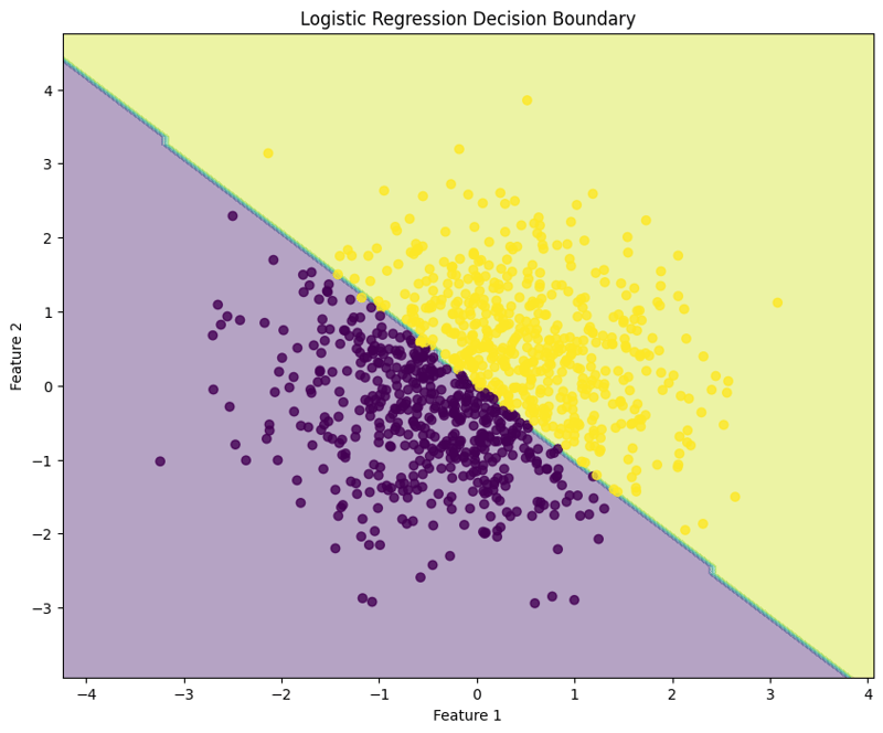
이 구조화된 접근 방식은 로지스틱 회귀를 구현하고 평가하는 방법을 보여 주며 이진 분류 작업에 대한 기능을 명확하게 이해할 수 있게 해줍니다. 결정 경계의 시각화는 모델의 예측을 해석하는 데 도움이 됩니다.

Logistic Regression (Multiclass Classification) Example

Logistic regression can also be applied to multiclass classification tasks. This example demonstrates how to implement logistic regression using synthetic data, evaluate the model's performance, and visualize the decision boundary for three classes.

Python Code Example

1. Import Libraries

import numpy as np
import matplotlib.pyplot as plt
from sklearn.model_selection import train_test_split
from sklearn.linear_model import LogisticRegression
from sklearn.metrics import accuracy_score, confusion_matrix, classification_report

This block imports the necessary libraries for data manipulation, plotting, and machine learning.

2. Generate Sample Data with 3 Classes

np.random.seed(42)  # For reproducibility
n_samples = 999  # Total number of samples
n_samples_per_class = 333  # Ensure this is exactly n_samples // 3

# Class 0: Top-left corner
X0 = np.random.randn(n_samples_per_class, 2) * 0.5 + [-2, 2]

# Class 1: Top-right corner
X1 = np.random.randn(n_samples_per_class, 2) * 0.5 + [2, 2]

# Class 2: Bottom center
X2 = np.random.randn(n_samples_per_class, 2) * 0.5 + [0, -2]

# Combine the data
X = np.vstack([X0, X1, X2])
y = np.hstack([np.zeros(n_samples_per_class), 
               np.ones(n_samples_per_class), 
               np.full(n_samples_per_class, 2)])

# Shuffle the dataset
shuffle_idx = np.random.permutation(n_samples)
X, y = X[shuffle_idx], y[shuffle_idx]

This block generates synthetic data for three classes located in different regions of the feature space.

3. Split the Dataset

X_train, X_test, y_train, y_test = train_test_split(X, y, test_size=0.2, random_state=42)

This block splits the dataset into training and testing sets for model evaluation.

4. Create and Train the Logistic Regression Model

model = LogisticRegression(random_state=42)
model.fit(X_train, y_train)

This block initializes the logistic regression model and trains it using the training dataset.

5. Make Predictions

y_pred = model.predict(X_test)

This block uses the trained model to make predictions on the test set.

6. Evaluate the Model

accuracy = accuracy_score(y_test, y_pred)
conf_matrix = confusion_matrix(y_test, y_pred)
class_report = classification_report(y_test, y_pred)

print(f"Accuracy: {accuracy:.4f}")
print("\nConfusion Matrix:")
print(conf_matrix)
print("\nClassification Report:")
print(class_report)

Output:

Accuracy: 1.0000

Confusion Matrix:
[[54  0  0]
 [ 0 65  0]
 [ 0  0 81]]

Classification Report:
              precision    recall  f1-score   support

         0.0       1.00      1.00      1.00        54
         1.0       1.00      1.00      1.00        65
         2.0       1.00      1.00      1.00        81

    accuracy                           1.00       200
   macro avg       1.00      1.00      1.00       200
weighted avg       1.00      1.00      1.00       200

This block calculates and prints the accuracy, confusion matrix, and classification report, providing insights into the model's performance.

7. Visualize the Decision Boundary

x_min, x_max = X[:, 0].min() - 1, X[:, 0].max() + 1
y_min, y_max = X[:, 1].min() - 1, X[:, 1].max() + 1
xx, yy = np.meshgrid(np.arange(x_min, x_max, 0.1),
                     np.arange(y_min, y_max, 0.1))
Z = model.predict(np.c_[xx.ravel(), yy.ravel()])
Z = Z.reshape(xx.shape)

plt.figure(figsize=(10, 8))
plt.contourf(xx, yy, Z, alpha=0.4, cmap='RdYlBu')
scatter = plt.scatter(X[:, 0], X[:, 1], c=y, cmap='RdYlBu', edgecolor='black')
plt.xlabel("Feature 1")
plt.ylabel("Feature 2")
plt.title("Multiclass Logistic Regression Decision Boundary")
plt.colorbar(scatter)
plt.show()

This block visualizes the decision boundaries created by the logistic regression model, illustrating how the model separates the three classes in the feature space.

Output:

This structured approach demonstrates how to implement and evaluate logistic regression for multiclass classification tasks, providing a clear understanding of its capabilities and the effectiveness of visualizing decision boundaries.

Evaluating Logistic Regression Model

Evaluating a logistic regression model involves assessing its performance in predicting binary or multiclass outcomes. Below are key methods for evaluation:

1. Performance Metrics

• Accuracy: The proportion of correctly classified instances out of the total instances. It provides a general sense of the model's performance.
  • Formula: Accuracy = (TP + TN) / (TP + TN + FP + FN)

  from sklearn.metrics import accuracy_score

  accuracy = accuracy_score(y_test, y_pred)
  print(f'Accuracy: {accuracy:.4f}')

• Confusion Matrix: A table that summarizes the performance of the classification model by showing the true positives (TP), true negatives (TN), false positives (FP), and false negatives (FN).

  from sklearn.metrics import confusion_matrix

  conf_matrix = confusion_matrix(y_test, y_pred)
  print("\nConfusion Matrix:")
  print(conf_matrix)

• Precision: Measures the accuracy of the positive predictions. It is the ratio of true positives to the sum of true and false positives.
  • Formula: Precision = TP / (TP + FP)

  from sklearn.metrics import precision_score

  precision = precision_score(y_test, y_pred, average='weighted')
  print(f'Precision: {precision:.4f}')

• Recall (Sensitivity): Measures the model's ability to identify all relevant instances (true positives). It is the ratio of true positives to the sum of true positives and false negatives.
  • Formula: Recall = TP / (TP + FN)

  from sklearn.metrics import recall_score

  recall = recall_score(y_test, y_pred, average='weighted')
  print(f'Recall: {recall:.4f}')

• F1 Score: The harmonic mean of precision and recall, providing a balance between the two metrics. It is useful when the class distribution is imbalanced.
  • Formula: F1 Score = 2 * (Precision * Recall) / (Precision + Recall)

  from sklearn.metrics import f1_score

  f1 = f1_score(y_test, y_pred, average='weighted')
  print(f'F1 Score: {f1:.4f}')

2. Cross-Validation

Cross-validation techniques provide a more reliable evaluation of model performance by assessing it across different subsets of the dataset.

• K-Fold Cross-Validation: The dataset is divided into k subsets, and the model is trained on k-1 subsets while validating on the remaining subset. This is repeated k times, and the average metric provides a robust evaluation.

  from sklearn.model_selection import KFold, cross_val_score

  kf = KFold(n_splits=5, shuffle=True, random_state=42)
  scores = cross_val_score(model, X, y, cv=kf, scoring='accuracy')
  print(f'Cross-Validation Accuracy: {np.mean(scores):.4f}')

• Stratified K-Fold Cross-Validation: Similar to K-Fold but ensures that each fold maintains the class distribution, which is particularly beneficial for imbalanced datasets.

  from sklearn.model_selection import StratifiedKFold

  skf = StratifiedKFold(n_splits=5)
  scores = cross_val_score(model, X, y, cv=skf, scoring='accuracy')
  print(f'Stratified K-Fold Cross-Validation Accuracy: {np.mean(scores):.4f}')

By utilizing these evaluation methods and cross-validation techniques, practitioners can gain insights into the effectiveness of their logistic regression model and its ability to generalize to unseen data.

Regularization in Logistic Regression

Regularization helps mitigate overfitting in logistic regression by adding a penalty term to the loss function, encouraging simpler models. The two primary forms of regularization in logistic regression are L1 regularization (Lasso) and L2 regularization (Ridge).

L2 정규화(능형 로지스틱 회귀)

개념: L2 정규화는 손실 함수에 계수 크기의 제곱에 해당하는 페널티를 추가합니다.

손실 함수: Ridge 로지스틱 회귀의 수정된 손실 함수는 다음과 같이 표현됩니다.

손실 = -Σ[yi * log(ŷi) + (1 - yi) * log(1 - ŷi)] + λ * Σ(wj^2)

장소:

• yi는 실제 클래스 라벨입니다.
• ŷi는 양성 클래스의 예측 확률입니다.
• wj는 모델 계수입니다.
• λ는 정규화 매개변수입니다.

효과:

• 능선 정규화는 계수를 0으로 축소하지만 제거하지는 않습니다. 모든 기능이 모델에 유지되므로 예측 변수가 많거나 다중 공선성이 있는 경우에 유용합니다.

L1 정규화(올가미 로지스틱 회귀)

개념: L1 정규화는 손실 함수에 계수 크기의 절대값과 동일한 페널티를 추가합니다.

손실 함수: Lasso 로지스틱 회귀의 수정된 손실 함수는 다음과 같이 표현할 수 있습니다.

손실 = -Σ[yi * log(ŷi) + (1 - yi) * log(1 - ŷi)] + λ * Σ|wj|

장소:

• yi는 실제 클래스 라벨입니다.
• ŷi는 양성 클래스의 예측 확률입니다.
• wj는 모델 계수입니다.
• λ는 정규화 매개변수입니다.

효과:

• Lasso 정규화는 일부 계수를 정확히 0으로 설정하여 변수 선택을 효과적으로 수행할 수 있습니다. 이는 해석 가능성이 필수적인 고차원 데이터 세트에 유리합니다.

로지스틱 회귀에 정규화 기술을 적용함으로써 실무자는 모델 일반화를 향상하고 편향-분산 균형을 효과적으로 관리할 수 있습니다.

위 내용은 로지스틱 회귀, 분류: 지도 머신러닝의 상세 내용입니다. 자세한 내용은 PHP 중국어 웹사이트의 기타 관련 기사를 참조하세요!