Python を使用してゼロから回帰木を手書きする

簡単にするために、ツリー ノードの作成に再帰を使用します。再帰は完全な実装ではありませんが、原理を説明するのに最も直感的です。

最初にライブラリをインポートします

import pandas as pd
import numpy as np
import matplotlib.pyplot as plt

まずトレーニング データを作成する必要があります。データには独立変数 (x) と従属変数 (y) があり、numpy を使用してガウス分布を追加します。相関値ノイズは数学的に次のように表現できます。

ここでノイズです。コードを以下に示します。

def f(x):
mu, sigma = 0, 1.5
return -x**2 + x + 5 + np.random.normal(mu, sigma, 1)
num_points = 300
np.random.seed(1)

x = np.random.uniform(-2, 5, num_points)
y = np.array( [f(i) for i in x] )
plt.scatter(x, y, s = 5)

回帰木

回帰木では、複数のノードからなる木を作成することで数値データを予測します。以下の図は、回帰ツリーのツリー構造の例を示しています。各ノードには、データを分割するために使用されるしきい値があります。

#一連のデータが与えられると、入力値は対応する仕様を通じてリーフ ノードに到達します。ノード M に到達するすべての入力値は、X のサブセットで表すことができます。数学的に、この状況を、指定された入力値がノード M に到達した場合は 1 を返し、それ以外の場合は 0 を与える関数の観点から表現してみましょう。

データを分割するしきい値を見つける: 各ステップで連続する 2 つのポイントを選択し、それらの平均を計算することにより、トレーニング データを反復処理します。計算された平均により、データが 2 つのしきい値に分割されます。

まず、特定の状況を示すためのランダムなしきい値を考えてみましょう。

threshold = 1.5
low = np.take(y, np.where(x < threshold))
high = np.take(y, np.where(x > threshold))
plt.scatter(x, y, s = 5, label = 'Data')
plt.plot([threshold]*2, [-16, 10], 'b--', label = 'Threshold line')
plt.plot([-2, threshold], [low.mean()]*2, 'r--', label = 'Left child prediction line')
plt.plot([threshold, 5], [high.mean()]*2, 'r--', label = 'Right child prediction line')
plt.plot([-2, 5], [y.mean()]*2, 'g--', label = 'Node prediction line')
plt.legend()

青い縦線は 1 つのしきい値を表します。これは任意の 2 点の平均であると想定され、後でデータを分割するために使用されます。

この問題に対する最初の予測は、すべてのトレーニング データ (y 軸) の平均 (緑色の水平線) です。そして、赤い 2 本の線は、作成される子ノードの予測です。

これらの平均値がいずれもデータを適切に表していないことは明らかですが、それらの違いも明らかです。マスター ノードの予測 (緑の線) はすべてのトレーニング データの平均値を取得し、これを 2 つの子ノードに分割します。 2 つの子ノードには独自の予測があります (赤線)。緑の線と比較すると、これら 2 つの子ノードは、対応するトレーニング データをよりよく表しています。回帰ツリーは、指定された停止値 (ノードが保持できる最小データ量) に達するまで、データを 2 つの部分に継続的に分割し、各ノードから 2 つの子ノードを作成します。これにより、ツリーの構築プロセスが早期に停止され、これを事前剪定ツリーと呼びます。

なぜ早期停止メカニズムがあるのですか?ノードの値が 1 つだけになるまで割り当てを続けると、各トレーニング データがそれ自体を予測することしかできない過学習シナリオが作成されます。

説明: モデルが完成すると、値の予測にルート ノードや中間ノードは使用されず、回帰ツリーのリーフ (ツリーの最後のノードになります) が使用されます。予測を立てるためです。

特定のしきい値のデータを最もよく表すしきい値を取得するには、残差二乗和を使用します。これは数学的に次のように定義できます。

# このステップがどのように機能するかを見てみましょう。

しきい値の SSR 値が計算されたので、最小の SSR 値を持つしきい値を使用できます。このしきい値を使用して、トレーニング データを 2 つ (低位部分と高位部分) に分割します。低位部分は左の子ノードの作成に使用され、高位部分は右の子ノードの作成に使用されます。

def SSR(r, y): 
return np.sum( (r - y)**2 )

SSRs, thresholds = [], []
for i in range(len(x) - 1):
threshold = x[i:i+2].mean()

low = np.take(y, np.where(x < threshold))
high = np.take(y, np.where(x > threshold))

guess_low = low.mean()
guess_high = high.mean()

SSRs.append(SSR(low, guess_low) + SSR(high, guess_high))
thresholds.append(threshold)

print('Minimum residual is: {:.2f}'.format(min(SSRs)))
print('Corresponding threshold value is: {:.4f}'.format(thresholds[SSRs.index(min(SSRs))]))

在进入下一步之前，我将使用pandas创建一个df，并创建一个用于寻找最佳阈值的方法。所有这些步骤都可以在没有pandas的情况下完成，这里使用他是因为比较方便。

df = pd.DataFrame(zip(x, y.squeeze()), columns = ['x', 'y'])
def find_threshold(df, plot = False):
SSRs, thresholds = [], []
for i in range(len(df) - 1):
threshold = df.x[i:i+2].mean()
low = df[(df.x <= threshold)]
high = df[(df.x > threshold)]
guess_low = low.y.mean()
guess_high = high.y.mean()
SSRs.append(SSR(low.y.to_numpy(), guess_low) + SSR(high.y.to_numpy(), guess_high))
thresholds.append(threshold)

if plot:
plt.scatter(thresholds, SSRs, s = 3)
plt.show()

return thresholds[SSRs.index(min(SSRs))]

创建子节点

在将数据分成两个部分后就可以为低值和高值找到单独的阈值。需要注意的是这里要增加一个停止条件;因为对于每个节点，属于该节点的数据集中的点会变少，所以我们为每个节点定义了最小数据点数量。如果不这样做，每个节点将只使用一个训练值进行预测，会导致过拟合。

可以递归地创建节点，我们定义了一个名为TreeNode的类，它将存储节点应该存储的每一个值。使用这个类我们首先创建根，同时计算它的阈值和预测值。然后递归地创建它的子节点，其中每个子节点类都存储在父类的left或right属性中。

在下面的create_nodes方法中，首先将给定的df分成两部分。然后检查是否有足够的数据单独创建左右节点。如果(对于其中任何一个)有足够的数据点，我们计算阈值并使用它创建一个子节点，用这个新节点作为树再次调用create_nodes方法。

class TreeNode():
def __init__(self, threshold, pred):
self.threshold = threshold
self.pred = pred
self.left = None
self.right = None
def create_nodes(tree, df, stop):
low = df[df.x <= tree.threshold]
high = df[df.x > tree.threshold]

if len(low) > stop:
threshold = find_threshold(low)
tree.left = TreeNode(threshold, low.y.mean())
create_nodes(tree.left, low, stop)

if len(high) > stop:
threshold = find_threshold(high)
tree.right = TreeNode(threshold, high.y.mean())
create_nodes(tree.right, high, stop)

threshold = find_threshold(df)
tree = TreeNode(threshold, df.y.mean())
create_nodes(tree, df, 5)

这个方法在第一棵树上进行了修改，因为它不需要返回任何东西。虽然递归函数通常不是这样写的(不返回)，但因为不需要返回值，所以当没有激活if语句时，不做任何操作。

在完成后可以检查此树结构，查看它是否创建了一些可以拟合数据的节点。 这里将手动选择第一个节点及其对根阈值的预测。

plt.scatter(x, y, s = 0.5, label = 'Data')
plt.plot([tree.threshold]*2, [-16, 10], 'r--', 
label = 'Root threshold')
plt.plot([tree.right.threshold]*2, [-16, 10], 'g--', 
label = 'Right node threshold')
plt.plot([tree.threshold, tree.right.threshold], 
[tree.right.left.pred]*2,
'g', label = 'Right node prediction')
plt.plot([tree.left.threshold]*2, [-16, 10], 'm--', 
label = 'Left node threshold')
plt.plot([tree.left.threshold, tree.threshold], 
[tree.left.right.pred]*2,
'm', label = 'Left node prediction')
plt.plot([tree.left.left.threshold]*2, [-16, 10], 'k--',
label = 'Second Left node threshold')
plt.legend()

这里看到了两个预测:

• 第一个左节点对高值的预测(高于其阈值)
• 第一个右节点对低值(低于其阈值)的预测

这里我手动剪切了预测线的宽度，因为如果给定的x值达到了这些节点中的任何一个，则将以属于该节点的所有x值的平均值表示，这也意味着没有其他x值参与 在该节点的预测中（希望有意义）。

这种树形结构远不止两个节点那么简单，所以我们可以通过如下调用它的子节点来检查一个特定的叶子节点。

tree.left.right.left.left

这当然意味着这里有一个向下4个子结点长的分支，但它可以在树的另一个分支上深入得多。

预测

我们可以创建一个预测方法来预测任何给定的值。

def predict(x):
curr_node = tree
result = None
while True:
if x <= curr_node.threshold:
if curr_node.left: curr_node = curr_node.left
else: 
break
elif x > curr_node.threshold:
if curr_node.right: curr_node = curr_node.right
else: 
break

return curr_node.pred

预测方法做的是沿着树向下，通过比较我们的输入和每个叶子的阈值。如果输入值大于阈值，则转到右叶，如果小于阈值，则转到左叶，以此类推，直到到达任何底部叶子节点。然后使用该节点自身的预测值进行预测，并与其阈值进行最后的比较。

使用x = 3进行测试(在创建数据时，可以使用上面所写的函数计算实际值。-3**2+3+5 = -1，这是期望值)，我们得到:

predict(3)
# -1.23741

计算误差

这里用相对平方误差验证数据

def RSE(y, g): 
return sum(np.square(y - g)) / sum(np.square(y - 1 / len(y)*sum(y)))
x_val = np.random.uniform(-2, 5, 50)
y_val = np.array( [f(i) for i in x_val] ).squeeze()
tr_preds = np.array( [predict(i) for i in df.x] )
val_preds = np.array( [predict(i) for i in x_val] )
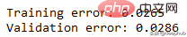
print('Training error: {:.4f}'.format(RSE(df.y, tr_preds)))
print('Validation error: {:.4f}'.format(RSE(y_val, val_preds)))

可以看到误差并不大，结果如下

概括的步骤

更深入的模型

一个更适合回归树模型的数据：因为我们的数据是多项式生成的数据，所以使用多项式回归模型可以更好地拟合。我们更换一下训练数据，把新函数设为

def f(x):
mu, sigma = 0, 0.5
if x < 3: return 1 + np.random.normal(mu, sigma, 1)
elif x >= 3 and x < 6: return 9 + np.random.normal(mu, sigma, 1)
elif x >= 6: return 5 + np.random.normal(mu, sigma, 1)

np.random.seed(1)

x = np.random.uniform(0, 10, num_points)
y = np.array( [f(i) for i in x] )
plt.scatter(x, y, s = 5)

在此数据集上运行了上面的所有相同过程，结果如下

比我们从多项式数据中获得的误差低。

最后共享一下上面动图的代码：

import pandas as pd
import numpy as np
import matplotlib.pyplot as plt
from matplotlib.animation import FuncAnimation
#===================================================Create Data
def f(x):
mu, sigma = 0, 1.5
return -x**2 + x + 5 + np.random.normal(mu, sigma, 1)
np.random.seed(1)

x = np.random.uniform(-2, 5, 300)
y = np.array( [f(i) for i in x] )
p = x.argsort()
x = x[p]
y = y[p]
#===================================================Calculate Thresholds
def SSR(r, y): #send numpy array
return np.sum( (r - y)**2 )
SSRs, thresholds = [], []
for i in range(len(x) - 1):
threshold = x[i:i+2].mean()

low = np.take(y, np.where(x < threshold))
high = np.take(y, np.where(x > threshold))

guess_low = low.mean()
guess_high = high.mean()

SSRs.append(SSR(low, guess_low) + SSR(high, guess_high))
thresholds.append(threshold)
#===================================================Animated Plot
fig, (ax1, ax2) = plt.subplots(2,1, sharex = True)
x_data, y_data = [], []
x_data2, y_data2 = [], []
ln, = ax1.plot([], [], 'r--')
ln2, = ax2.plot(thresholds, SSRs, 'ro', markersize = 2)
line = [ln, ln2]
def init():
ax1.scatter(x, y, s = 3)
ax1.title.set_text('Trying Different Thresholds')
ax2.title.set_text('Threshold vs SSR')
ax1.set_ylabel('y values')
ax2.set_xlabel('Threshold')
ax2.set_ylabel('SSR')
return line
def update(frame):
x_data = [x[frame:frame+2].mean()] * 2
y_data = [min(y), max(y)]
line[0].set_data(x_data, y_data)
x_data2.append(thresholds[frame])
y_data2.append(SSRs[frame])
line[1].set_data(x_data2, y_data2)
return line
ani = FuncAnimation(fig, update, frames = 298,
init_func = init, blit = True)
plt.show()

以上がPython を使用してゼロから回帰木を手書きするの詳細内容です。詳細については、PHP 中国語 Web サイトの他の関連記事を参照してください。