ロジスティック回帰、分類: 教師あり機械学習

分類とは何ですか?

定義と目的

分類 は、機械学習とデータ サイエンスでデータを事前定義されたクラスまたはラベルに分類するために使用される教師あり学習手法です。これには、入力データ ポイントをその特徴に基づいていくつかの離散カテゴリの 1 つに割り当てるモデルのトレーニングが含まれます。分類の主な目的は、新しい未知のデータ ポイントのクラスまたはカテゴリを正確に予測することです。

主な目的:

• 予測: 事前定義されたクラスの 1 つに新しいデータ ポイントを割り当てます。
• 推定: データ ポイントが特定のクラスに属する確率を決定します。
• 関係を理解する: データ ポイントのクラスを予測する際にどの特徴が重要であるかを特定します。

分類の種類

1.バイナリ分類

• 説明: データを 2 つのクラスのいずれかに分類します。
  • 例: スパム検出 (スパムかどうか)、病気の診断 (病気か病気ではないか)。
  • 目的: 2 つの異なるクラスを区別します。

2.マルチクラス分類

• 説明: データを 3 つ以上のクラスの 1 つに分類します。
  • 例: 手書きの数字認識 (0 ～ 9 の数字)、花の種類の分類 (複数の種)。
  • 目的: 予測するクラスが 3 つ以上ある問題を処理します。

線形分類子とは何ですか?

線形分類器 は、線形決定境界を使用して特徴空間内の異なるクラスを分離する分類アルゴリズムのカテゴリです。線形方程式を通じて入力特徴を組み合わせることによって予測を行い、通常は特徴とターゲット クラス ラベルの間の関係を表します。線形分類器の主な目的は、特徴空間を個別のクラスに分割する超平面を見つけて、データ ポイントを効率的に分類することです。

ロジスティック回帰

定義と目的

ロジスティック回帰 は、機械学習とデータ サイエンスのバイナリ分類タスクに使用される統計手法です。これは線形分類器の一部であり、データをロジスティック曲線に当てはめることによってイベントの発生確率を予測するという点で線形回帰とは異なります。

主な目的:

• バイナリ分類: バイナリ結果 (はい/いいえ、真/偽など) を予測します。
• 確率推定: 入力変数に基づいてイベントが発生する確率を推定します。
• 決定境界: データをさまざまなクラスに分類するためのしきい値を決定します。

ロジスティック回帰モデル

1.ロジスティック関数（シグモイド関数）

• 説明: ロジスティック関数は、実数値の入力を 0 から 1 までの値に変換し、確率のモデリングに適しています。
  • 方程式: σ(z) = 1 / (1 + e^(-z))
  • 目的: 入力値を確率にマッピングします。

2.ロジスティック回帰式

• 説明: ロジスティック回帰モデルは、入力変数の線形結合にロジスティック関数を適用します。
  • 方程式: P(y=1|x) = σ(w0 + w1x1 + w2x2 + ... + wnxn)
  • 目的: 入力変数 x が与えられた場合のバイナリ結果 y=1 の確率 P(y=1|x) を予測します。

最尤推定 (MLE)

MLE は、モデルに与えられたデータを観察する可能性を最大化することにより、ロジスティック回帰モデルのパラメーター (係数) を推定するために使用されます。

方程式: 対数尤度関数の最大化には、データを観測する確率を最大化するパラメーターを見つけることが含まれます。

ロジスティック回帰におけるコスト関数と損失の最小化

コスト関数

ロジスティック回帰のコスト関数は、予測された確率と実際のクラスラベルの差を測定します。目標は、この関数を最小化してモデルの予測精度を向上させることです。

対数損失 (バイナリクロスエントロピー):
対数損失関数は、バイナリ分類タスクのロジスティック回帰でよく使用されます。

対数損失 = -(1/n) * Σ [y * log(ŷ) + (1 - y) * log(1 - ŷ)]

ここで:

• y は実際のクラス ラベル (0 または 1)、
• ŷ はクラス ラベルの予測確率です。
• n はデータポイントの数です。

対数損失により、実際のクラス ラベルからかけ離れた予測にペナルティが課され、モデルが正確な確率を生成することが促進されます。

損失の最小化（最適化）

ロジスティック回帰における

損失の最小化には、コスト関数値を最小化するモデル パラメーターの値を見つけることが含まれます。このプロセスは最適化としても知られています。ロジスティック回帰における損失を最小化するための最も一般的な方法は、勾配降下法 アルゴリズムです。

勾配降下法

勾配降下法は、ロジスティック回帰のコスト関数を最小化するために使用される反復最適化アルゴリズムです。コスト関数の最急降下方向にモデル パラメーターを調整します。

勾配降下のステップ:

1. パラメータの初期化: モデル パラメータの初期値 (係数 w0、w1、...、wn など) から開始します。

2. 勾配の計算: 各パラメーターに関してコスト関数の勾配を計算します。勾配はコスト関数の偏導関数です。

3. パラメータの更新: グラデーションの反対方向にパラメータを調整します。調整は学習率 (α) によって制御され、最小値に向けて実行されるステップのサイズが決まります。

4. Repeat: コスト関数が最小値に収束する (または事前に定義された反復回数に達する) までプロセスを繰り返します。

パラメータ更新ルール:
各パラメータ wj について:
wj = wj - α * (∂/∂wj) 対数損失

ここで:

• α は学習率です。
• (∂/∂wj) 対数損失は、wj に関する対数損失の偏導関数です。

wj に関する対数損失の偏導関数は次のように計算できます。
(∂/∂wj) 対数損失 = -(1/n) * Σ [ (yi - ŷi) * xij / (ŷi * (1 - ŷi)) ]

ここで:

• xij は、i 番目のデータポイントの j 番目の独立変数の値です。
• ŷi は、i 番目のデータ ポイントのクラス ラベルの予測確率です。

ロジスティック回帰 (二項分類) の例

ロジスティック回帰は、バイナリ分類タスクに使用される手法であり、特定の入力が特定のクラスに属する確率をモデル化します。この例では、合成データを使用してロジスティック回帰を実装し、モデルのパフォーマンスを評価し、決定境界を視覚化する方法を示します。

Python コード例

1.ライブラリをインポート

import numpy as np
import matplotlib.pyplot as plt
from sklearn.model_selection import train_test_split
from sklearn.linear_model import LogisticRegression
from sklearn.metrics import accuracy_score, confusion_matrix, classification_report

このブロックは、データ操作、プロット、機械学習に必要なライブラリをインポートします。

2.サンプルデータの生成

np.random.seed(42)  # For reproducibility
X = np.random.randn(1000, 2)
y = (X[:, 0] + X[:, 1] > 0).astype(int)

このブロックは 2 つの特徴を持つサンプル データを生成します。ターゲット変数 y は特徴の合計が 0 より大きいかどうかに基づいて定義され、バイナリ分類シナリオをシミュレートします。

3.データセットを分割します

X_train, X_test, y_train, y_test = train_test_split(X, y, test_size=0.2, random_state=42)

このブロックは、モデル評価のためにデータセットをトレーニング セットとテスト セットに分割します。

4.ロジスティック回帰モデルの作成とトレーニング

model = LogisticRegression(random_state=42)
model.fit(X_train, y_train)

このブロックはロジスティック回帰モデルを初期化し、トレーニング データセットを使用してトレーニングします。

5.予測を立てる

y_pred = model.predict(X_test)

このブロックは、トレーニングされたモデルを使用してテスト セットで予測を行います。

6.モデルを評価する

accuracy = accuracy_score(y_test, y_pred)
conf_matrix = confusion_matrix(y_test, y_pred)
class_report = classification_report(y_test, y_pred)

print(f"Accuracy: {accuracy:.4f}")
print("\nConfusion Matrix:")
print(conf_matrix)
print("\nClassification Report:")
print(class_report)

出力:

Accuracy: 0.9950

Confusion Matrix:
[[ 92   0]
 [  1 107]]

Classification Report:
              precision    recall  f1-score   support

           0       0.99      1.00      0.99        92
           1       1.00      0.99      1.00       108

    accuracy                           0.99       200
   macro avg       0.99      1.00      0.99       200
weighted avg       1.00      0.99      1.00       200

このブロックは、精度、混同行列、分類レポートを計算して出力し、モデルのパフォーマンスに関する洞察を提供します。

7.意思決定の境界線を可視化する

x_min, x_max = X[:, 0].min() - 1, X[:, 0].max() + 1
y_min, y_max = X[:, 1].min() - 1, X[:, 1].max() + 1
xx, yy = np.meshgrid(np.arange(x_min, x_max, 0.1),
                     np.arange(y_min, y_max, 0.1))
Z = model.predict(np.c_[xx.ravel(), yy.ravel()])
Z = Z.reshape(xx.shape)

plt.figure(figsize=(10, 8))
plt.contourf(xx, yy, Z, alpha=0.4)
plt.scatter(X[:, 0], X[:, 1], c=y, alpha=0.8)
plt.xlabel("Feature 1")
plt.ylabel("Feature 2")
plt.title("Logistic Regression Decision Boundary")
plt.show()

このブロックは、ロジスティック回帰モデルによって作成された決定境界を視覚化し、モデルが特徴空間内の 2 つのクラスをどのように分離するかを示します。

出力:

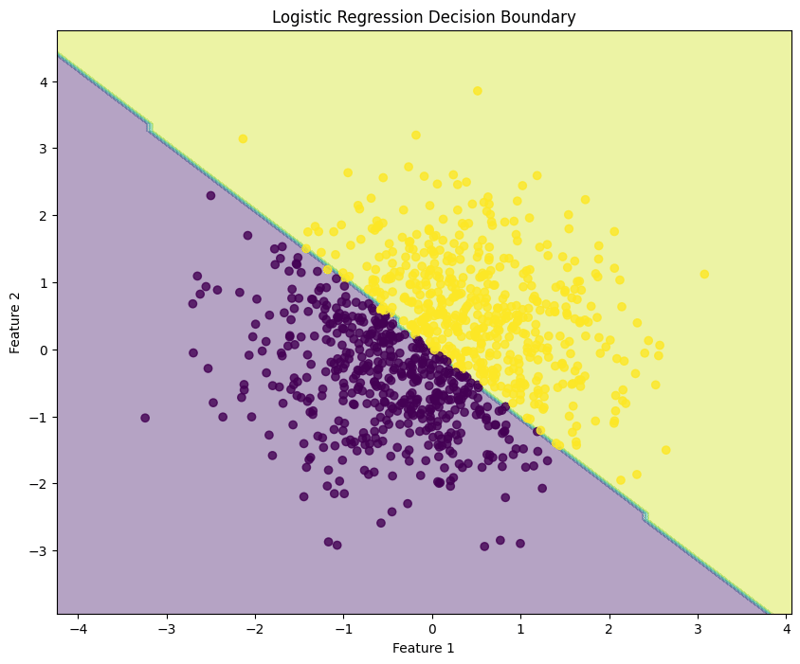
この構造化されたアプローチは、ロジスティック回帰を実装および評価する方法を示し、バイナリ分類タスクに対するロジスティック回帰の機能を明確に理解できるようにします。決定境界の視覚化は、モデルの予測の解釈に役立ちます。

Logistic Regression (Multiclass Classification) Example

Logistic regression can also be applied to multiclass classification tasks. This example demonstrates how to implement logistic regression using synthetic data, evaluate the model's performance, and visualize the decision boundary for three classes.

Python Code Example

1. Import Libraries

import numpy as np
import matplotlib.pyplot as plt
from sklearn.model_selection import train_test_split
from sklearn.linear_model import LogisticRegression
from sklearn.metrics import accuracy_score, confusion_matrix, classification_report

This block imports the necessary libraries for data manipulation, plotting, and machine learning.

2. Generate Sample Data with 3 Classes

np.random.seed(42)  # For reproducibility
n_samples = 999  # Total number of samples
n_samples_per_class = 333  # Ensure this is exactly n_samples // 3

# Class 0: Top-left corner
X0 = np.random.randn(n_samples_per_class, 2) * 0.5 + [-2, 2]

# Class 1: Top-right corner
X1 = np.random.randn(n_samples_per_class, 2) * 0.5 + [2, 2]

# Class 2: Bottom center
X2 = np.random.randn(n_samples_per_class, 2) * 0.5 + [0, -2]

# Combine the data
X = np.vstack([X0, X1, X2])
y = np.hstack([np.zeros(n_samples_per_class), 
               np.ones(n_samples_per_class), 
               np.full(n_samples_per_class, 2)])

# Shuffle the dataset
shuffle_idx = np.random.permutation(n_samples)
X, y = X[shuffle_idx], y[shuffle_idx]

This block generates synthetic data for three classes located in different regions of the feature space.

3. Split the Dataset

X_train, X_test, y_train, y_test = train_test_split(X, y, test_size=0.2, random_state=42)

This block splits the dataset into training and testing sets for model evaluation.

4. Create and Train the Logistic Regression Model

model = LogisticRegression(random_state=42)
model.fit(X_train, y_train)

This block initializes the logistic regression model and trains it using the training dataset.

5. Make Predictions

y_pred = model.predict(X_test)

This block uses the trained model to make predictions on the test set.

6. Evaluate the Model

accuracy = accuracy_score(y_test, y_pred)
conf_matrix = confusion_matrix(y_test, y_pred)
class_report = classification_report(y_test, y_pred)

print(f"Accuracy: {accuracy:.4f}")
print("\nConfusion Matrix:")
print(conf_matrix)
print("\nClassification Report:")
print(class_report)

Output:

Accuracy: 1.0000

Confusion Matrix:
[[54  0  0]
 [ 0 65  0]
 [ 0  0 81]]

Classification Report:
              precision    recall  f1-score   support

         0.0       1.00      1.00      1.00        54
         1.0       1.00      1.00      1.00        65
         2.0       1.00      1.00      1.00        81

    accuracy                           1.00       200
   macro avg       1.00      1.00      1.00       200
weighted avg       1.00      1.00      1.00       200

This block calculates and prints the accuracy, confusion matrix, and classification report, providing insights into the model's performance.

7. Visualize the Decision Boundary

x_min, x_max = X[:, 0].min() - 1, X[:, 0].max() + 1
y_min, y_max = X[:, 1].min() - 1, X[:, 1].max() + 1
xx, yy = np.meshgrid(np.arange(x_min, x_max, 0.1),
                     np.arange(y_min, y_max, 0.1))
Z = model.predict(np.c_[xx.ravel(), yy.ravel()])
Z = Z.reshape(xx.shape)

plt.figure(figsize=(10, 8))
plt.contourf(xx, yy, Z, alpha=0.4, cmap='RdYlBu')
scatter = plt.scatter(X[:, 0], X[:, 1], c=y, cmap='RdYlBu', edgecolor='black')
plt.xlabel("Feature 1")
plt.ylabel("Feature 2")
plt.title("Multiclass Logistic Regression Decision Boundary")
plt.colorbar(scatter)
plt.show()

This block visualizes the decision boundaries created by the logistic regression model, illustrating how the model separates the three classes in the feature space.

Output:

This structured approach demonstrates how to implement and evaluate logistic regression for multiclass classification tasks, providing a clear understanding of its capabilities and the effectiveness of visualizing decision boundaries.

Evaluating Logistic Regression Model

Evaluating a logistic regression model involves assessing its performance in predicting binary or multiclass outcomes. Below are key methods for evaluation:

1. Performance Metrics

• Accuracy: The proportion of correctly classified instances out of the total instances. It provides a general sense of the model's performance.
  • Formula: Accuracy = (TP + TN) / (TP + TN + FP + FN)

  from sklearn.metrics import accuracy_score

  accuracy = accuracy_score(y_test, y_pred)
  print(f'Accuracy: {accuracy:.4f}')

• Confusion Matrix: A table that summarizes the performance of the classification model by showing the true positives (TP), true negatives (TN), false positives (FP), and false negatives (FN).

  from sklearn.metrics import confusion_matrix

  conf_matrix = confusion_matrix(y_test, y_pred)
  print("\nConfusion Matrix:")
  print(conf_matrix)

• Precision: Measures the accuracy of the positive predictions. It is the ratio of true positives to the sum of true and false positives.
  • Formula: Precision = TP / (TP + FP)

  from sklearn.metrics import precision_score

  precision = precision_score(y_test, y_pred, average='weighted')
  print(f'Precision: {precision:.4f}')

• Recall (Sensitivity): Measures the model's ability to identify all relevant instances (true positives). It is the ratio of true positives to the sum of true positives and false negatives.
  • Formula: Recall = TP / (TP + FN)

  from sklearn.metrics import recall_score

  recall = recall_score(y_test, y_pred, average='weighted')
  print(f'Recall: {recall:.4f}')

• F1 Score: The harmonic mean of precision and recall, providing a balance between the two metrics. It is useful when the class distribution is imbalanced.
  • Formula: F1 Score = 2 * (Precision * Recall) / (Precision + Recall)

  from sklearn.metrics import f1_score

  f1 = f1_score(y_test, y_pred, average='weighted')
  print(f'F1 Score: {f1:.4f}')

2. Cross-Validation

Cross-validation techniques provide a more reliable evaluation of model performance by assessing it across different subsets of the dataset.

• K-Fold Cross-Validation: The dataset is divided into k subsets, and the model is trained on k-1 subsets while validating on the remaining subset. This is repeated k times, and the average metric provides a robust evaluation.

  from sklearn.model_selection import KFold, cross_val_score

  kf = KFold(n_splits=5, shuffle=True, random_state=42)
  scores = cross_val_score(model, X, y, cv=kf, scoring='accuracy')
  print(f'Cross-Validation Accuracy: {np.mean(scores):.4f}')

• Stratified K-Fold Cross-Validation: Similar to K-Fold but ensures that each fold maintains the class distribution, which is particularly beneficial for imbalanced datasets.

  from sklearn.model_selection import StratifiedKFold

  skf = StratifiedKFold(n_splits=5)
  scores = cross_val_score(model, X, y, cv=skf, scoring='accuracy')
  print(f'Stratified K-Fold Cross-Validation Accuracy: {np.mean(scores):.4f}')

By utilizing these evaluation methods and cross-validation techniques, practitioners can gain insights into the effectiveness of their logistic regression model and its ability to generalize to unseen data.

Regularization in Logistic Regression

Regularization helps mitigate overfitting in logistic regression by adding a penalty term to the loss function, encouraging simpler models. The two primary forms of regularization in logistic regression are L1 regularization (Lasso) and L2 regularization (Ridge).

L2 正則化 (リッジ ロジスティック回帰)

コンセプト: L2 正則化は、係数の大きさの 2 乗に等しいペナルティを損失関数に追加します。

損失関数: リッジ ロジスティック回帰の修正損失関数は次のように表されます:

損失 = -Σ[yi * log(ŷi) + (1 - yi) * log(1 - ŷi)] + λ * Σ(wj^2)

場所:

• yi は実際のクラスラベルです。
• ŷi は陽性クラスの予測確率です。
• wj はモデル係数です。
• λ は正則化パラメータです。

効果:

• リッジ正則化は係数をゼロに向かって縮小しますが、係数を削除しません。すべての特徴がモデル内に残るため、多くの予測子または多重共線性があるケースに有益です。

L1 正則化 (ラッソ ロジスティック回帰)

コンセプト: L1 正則化は、係数の大きさの絶対値に等しいペナルティを損失関数に追加します。

損失関数: Lasso ロジスティック回帰の修正損失関数は次のように表すことができます:

損失 = -Σ[yi * log(ŷi) + (1 - yi) * log(1 - ŷi)] + λ * Σ|wj|

場所:

• yi は実際のクラスラベルです。
• ŷi は陽性クラスの予測確率です。
• wj はモデル係数です。
• λ は正則化パラメータです。

効果:

• Lasso 正則化では、一部の係数を正確に 0 に設定して、変数選択を効果的に実行できます。これは、解釈可能性が重要な高次元データセットで有利です。

ロジスティック回帰に正則化手法を適用することで、実践者はモデルの一般化を強化し、バイアスと分散のトレードオフを効果的に管理できます。

以上がロジスティック回帰、分類: 教師あり機械学習の詳細内容です。詳細については、PHP 中国語 Web サイトの他の関連記事を参照してください。