php Editor Strawberry’s two methods for finding duplicate data in Excel are conditional formatting and data filtering. Through conditional formatting, duplicate data can be quickly marked and visually differentiated; through data filtering, duplicate data can be filtered out or deleted, helping users easily process duplicate information in Excel tables. These two methods are flexible and simple, suitable for data processing needs in different scenarios, and improve work efficiency.
1. We first select the data you want to find. If it is a different worksheet, then you need to copy Table 1 and press the CTRL plus key to insert it next to Table 2. The reason for this Yes, only by combining the two tables can we better find duplicate data in the two tables.

2. After combining the two tables, we need to select these two columns of data, that is, select the range where the repeated data is located.
3. After selecting it, you can click the [Conditional Formatting] option in the toolbar on the Home tab.
4. Then a drop-down list will appear. We need to click [Highlight Cell Rules] in the drop-down list, and then select [Duplicate Value].
5. Then an options page will pop up. We need to select [Repeat] in the pop-up interface and then adjust the color of the table according to our favorite color, and finally click OK. After clicking OK, the duplicate places will be found.

If you still want to delete these data separately, you need to click the [Data tab] first, and then you need to find [Delete Duplicates] and click [Delete Duplicates] ] Then all duplicate data can be easily deleted. The color can also be set freely. Data with the same color is a duplicate value.

The above is the detailed content of Two methods to find duplicate data in Excel. For more information, please follow other related articles on the PHP Chinese website!
 How to make a histogram in ExcelApr 22, 2025 am 10:33 AM
This tutorial explores three distinct methods for creating histograms in Excel: leveraging the Analysis ToolPak's Histogram tool, employing the FREQUENCY or COUNTIFS functions, and utilizing PivotCharts. While creating basic charts in Excel is strai
 Outlook signature: how to make, add and changeApr 22, 2025 am 09:54 AM
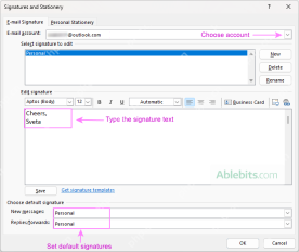
This comprehensive guide provides step-by-step instructions for creating and managing professional email signatures in Microsoft Outlook. Learn how to craft compelling signatures with images, clickable links, and more, across all Outlook versions (i
 Excel SUM formula to total a column, rows or only visible cellsApr 22, 2025 am 09:17 AM
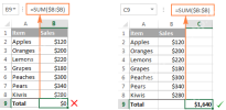
This tutorial demonstrates how to calculate sums in Excel using the AutoSum feature and custom SUM formulas for columns, rows, and selected ranges. It also covers summing only visible cells, calculating running totals, summing across multiple sheets
 How to AutoSum in ExcelApr 22, 2025 am 09:05 AM
This concise guide explains Excel's AutoSum feature and its efficient uses. Learn to quickly sum columns, rows, or visible cells, and troubleshoot common AutoSum issues. Excel's SUM function is incredibly popular, prompting Microsoft to include a ded
 Excel Switch function – the compact form of nested IF statementApr 22, 2025 am 09:04 AM
This article introduces the Excel SWITCH function, explaining its syntax and demonstrating its use in simplifying complex nested IF statements. If you've struggled with lengthy nested IF formulas, the SWITCH function offers a significant time-saving
 How to do a running total in Excel (Cumulative Sum formula)Apr 21, 2025 am 11:16 AM
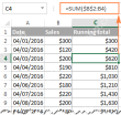
This concise guide demonstrates how to efficiently calculate running totals (cumulative sums) in Excel using a SUM formula with strategically placed absolute and relative cell references. A running total displays the accumulated sum of a dataset as
 Excel LEN function: count characters in cellApr 21, 2025 am 10:10 AM
Are you looking for an Excel formula to count characters in a cell? If so, then you have certainly landed up on the right page. This short tutorial will teach you how you can use the LEN function to count characters in Excel, with or with
 How to count words in Excel - formula examplesApr 21, 2025 am 09:59 AM
This tutorial demonstrates how to count words in Excel using a combination of the LEN, SUBSTITUTE, and TRIM functions. It offers both case-sensitive and case-insensitive formulas for counting total words or specific words/text within a cell or range


Hot AI Tools

Undresser.AI Undress
AI-powered app for creating realistic nude photos

AI Clothes Remover
Online AI tool for removing clothes from photos.

Undress AI Tool
Undress images for free

Clothoff.io
AI clothes remover

Video Face Swap
Swap faces in any video effortlessly with our completely free AI face swap tool!

Hot Article

Hot Tools

Notepad++7.3.1
Easy-to-use and free code editor

Dreamweaver Mac version
Visual web development tools

ZendStudio 13.5.1 Mac
Powerful PHP integrated development environment

SAP NetWeaver Server Adapter for Eclipse
Integrate Eclipse with SAP NetWeaver application server.

DVWA
Damn Vulnerable Web App (DVWA) is a PHP/MySQL web application that is very vulnerable. Its main goals are to be an aid for security professionals to test their skills and tools in a legal environment, to help web developers better understand the process of securing web applications, and to help teachers/students teach/learn in a classroom environment Web application security. The goal of DVWA is to practice some of the most common web vulnerabilities through a simple and straightforward interface, with varying degrees of difficulty. Please note that this software


