


php Xiaobian Yuzai will introduce to you how to use conditional formatting in Excel today. Conditional formatting is a very practical function in Excel. It can automatically format cells according to set conditions, making the data more intuitive and clear. By using conditional formatting appropriately, you can make your data easier to understand and analyze. Next, we will introduce the use of conditional formatting in detail to help you better use Excel for data processing and presentation.
1. This lesson explains the introduction of excel-conditional formatting

2. Here we explain the main content of this lesson, as shown in the figure .

3. We open the project file of this lesson and conduct a preview, as shown in the figure.

#4. We find a table default in [Apply Table Format], as shown in the figure.

#5. Then we select the content in the table, as shown in the figure.

#6. Select the content and open [Create Pivot Table], as shown in the figure.

#7. We check some of the content in the preset on the right, as shown in the picture.

#8. Then click [Conditional Formatting] to make a setting, as shown in the figure.

9. In the [Equal] setting, we make a setting adjustment, as shown in the figure.

10. Continue to select a content in [Edit Format Rules], as shown in the figure.

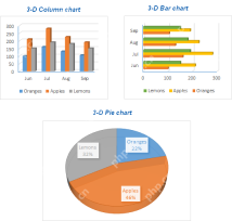
#11. Open the chart on another page and start explaining, as shown in the figure.

#12. If we double-click one of the columns, we can see the functions inside and give an explanation, as shown in the figure.

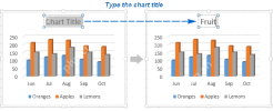
13. In the [Design] above, we open the chart title preset, as shown in the figure.

14. Then we load a picture preset, as shown in the picture.

#15. We make a setting adjustment in the parameters on the right, as shown in the figure.

16. Click on the next table to start an explanation, as shown in the picture.

#17. Select any column and enter an [=] sign and click on two of the contents, as shown in the picture.

#18. Use Format Painter to make a format adjustment, as shown in the figure.

19. Then we open the [Conditional Formatting Rule Manager] to make an adjustment, as shown in the figure.

#20. Open [Edit Format Rules] to make a setting adjustment, as shown in the figure.

21. Thank you for watching.

#So, how to use conditional formatting in excel format will be introduced here. I have to say that excel is very practical, and you will naturally remember the frequently used skills and functions if you use them more. But no matter how many times you learn the skills and functions that you rarely use, you will completely forget them if you don’t use them for three months. So practice the required skills more!
The above is the detailed content of How to use conditional formatting in excel. For more information, please follow other related articles on the PHP Chinese website!

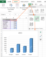
 How to make a chart (graph) in Excel and save it as templateApr 28, 2025 am 09:31 AM
This Excel charting tutorial provides a comprehensive guide to creating and customizing graphs within Microsoft Excel. Learn to visualize data effectively, from basic chart creation to advanced techniques. Everyone uses Excel charts to visualize dat
 Excel charts: add title, customize chart axis, legend and data labelsApr 28, 2025 am 09:18 AM
After you have created a chart in Excel, what's the first thing you usually want to do with it? Make the graph look exactly the way you've pictured it in your mind! In modern versions of Excel, customizing charts is easy and fun. Microsof
 Using Excel REPLACE and SUBSTITUTE functions - formula examplesApr 28, 2025 am 09:16 AM
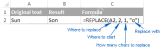
This tutorial demonstrates the Excel REPLACE and SUBSTITUTE functions with practical examples. Learn how to use REPLACE with text, numbers, and dates, and how to nest multiple REPLACE or SUBSTITUTE functions within a single formula. Last week, we ex
 Excel FIND and SEARCH functions with formula examplesApr 28, 2025 am 09:09 AM
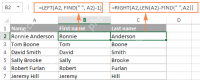
This tutorial details the syntax and advanced applications of Excel's FIND and SEARCH functions. Previous articles covered the basic Find and Replace dialog; this expands on using Excel to automatically locate and extract data based on specified cri
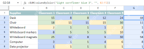 Count & sum cells by color in Google SheetsApr 28, 2025 am 09:04 AM
Google Sheets lacks built-in functions for summarizing data based on cell color. To overcome this, custom functions are provided that consider both font and background colors for basic calculations, enabling color-based summing and counting. These
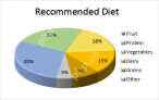 How to make a pie chart in ExcelApr 27, 2025 am 09:37 AM
This Excel pie chart tutorial guides you through creating and customizing pie charts. Learn to build effective pie charts, avoiding common pitfalls. Pie charts, also called circular graphs, visually represent proportions of a whole. Each slice repr
 How to create a chart in Excel from multiple sheetsApr 27, 2025 am 09:22 AM
This tutorial shows how to create and modify Excel charts from data across multiple worksheets. Previously, we covered basic charting; this expands on that by addressing the common question of combining data from different sheets. Creating Charts fr
 Why use $ in Excel formula: relative & absolute cell referenceApr 27, 2025 am 09:13 AM
The dollar sign ($) in cell references in Excel formulas often confuses users, but its principle is simple. The dollar sign has only one function in Excel cell references: it tells Excel whether to change the reference when copying a formula to another cell. This tutorial will explain this feature in detail. The importance of Excel cell reference cannot be overemphasized. Understand the difference between absolute, relative, and mixed citations, and you've mastered half of the power of Excel formulas and functions. You may have seen the dollar sign ($) in the Excel formula and want to know what it is. In fact, you can refer to the same cell in four different ways, such as A1, $A


Hot AI Tools

Undresser.AI Undress
AI-powered app for creating realistic nude photos

AI Clothes Remover
Online AI tool for removing clothes from photos.

Undress AI Tool
Undress images for free

Clothoff.io
AI clothes remover

Video Face Swap
Swap faces in any video effortlessly with our completely free AI face swap tool!

Hot Article
Hot Tools

MantisBT
Mantis is an easy-to-deploy web-based defect tracking tool designed to aid in product defect tracking. It requires PHP, MySQL and a web server. Check out our demo and hosting services.

EditPlus Chinese cracked version
Small size, syntax highlighting, does not support code prompt function

SublimeText3 Chinese version
Chinese version, very easy to use

ZendStudio 13.5.1 Mac
Powerful PHP integrated development environment

SecLists
SecLists is the ultimate security tester's companion. It is a collection of various types of lists that are frequently used during security assessments, all in one place. SecLists helps make security testing more efficient and productive by conveniently providing all the lists a security tester might need. List types include usernames, passwords, URLs, fuzzing payloads, sensitive data patterns, web shells, and more. The tester can simply pull this repository onto a new test machine and he will have access to every type of list he needs.

