

 Technology peripheralsAITrajectory generation under soft and hard constraints: detailed explanation of theory and code
Trajectory generation under soft and hard constraints: detailed explanation of theory and code

Code of this project:
github.com/liangwq/robot_motion_planing
Soft and hard constraints in trajectory constraints
Previous articles As already introduced, the essence of trajectory constraints is to perform constrained trajectory fitting. The input is the waypoint list, and there are two types of constraints: hard constraints and soft constraints. The so-called hard constraints correspond to the mathematical form of the cost function, and the hard constraints correspond to the constraint conditions of the optimization autumn. Corresponding to the physical meaning, in order to obtain a safe trajectory for the robot to walk:
- The way to push the trajectory away from the obstacles through the cost function
- gives the distance between the obstacles Walkable convex hull corridor, through hard constraints, the robot trajectory must walk in the convex hull corridor


The above picture shows The mathematical framework for solving Bezier curve fitting under soft and hard constraints, and how to convert various constraints into cost functions for mathematical solution (soft constraints) or constraints for solution (soft constraints). image.png

#The above are examples of several expressions of commonly used cost function constraints. image.png
Bezier curve fitting trajectory
An article has already introduced the various advantages of Bezier curve fitting:
- Endpoint interpolation. A Bezier curve always starts from the first control point, ends at the last control point, and does not pass through any other control points.
- Convex hull. A Bezier curve ( ) is made up of a set of control points and is completely constrained within the convex hull defined by all of those control points.
- Speed curve. The derivative curve ′( ) of the Bezier curve ( ) is called the velocity curve, which is also a Bezier curve defined by a control point, where the control point is ∙ ( 1− ), where is the order.
- Fixed time interval. Bezier curves are always defined on [0,1].

Fig1. A section of trajectory is fitted with a bezier curve image.png

The two expressions above The code implementation corresponding to the formula is as follows:
def bernstein_poly(n, i, t):"""Bernstein polynom.:param n: (int) polynom degree:param i: (int):param t: (float):return: (float)"""return scipy.special.comb(n, i) * t ** i * (1 - t) ** (n - i)def bezier(t, control_points):"""Return one point on the bezier curve.:param t: (float) number in [0, 1]:param control_points: (numpy array):return: (numpy array) Coordinates of the point"""n = len(control_points) - 1return np.sum([bernstein_poly(n, i, t) * control_points[i] for i in range(n + 1)], axis=0)
To use a Bezier curve to represent a curve, the expression and code implementation have been given above. What is missing now is to give the control points, bring the control points in and use Bezier Curve expression to calculate the coordinates of the points that need to be drawn in the given end point and end point. The following code gives the Bezier curve implementation of 4 control points and 6 control points; in order to draw the curve, 170 online points need to be calculated. The code is as follows:
def calc_4points_bezier_path(sx, sy, syaw, ex, ey, eyaw, offset):"""Compute control points and path given start and end position.:param sx: (float) x-coordinate of the starting point:param sy: (float) y-coordinate of the starting point:param syaw: (float) yaw angle at start:param ex: (float) x-coordinate of the ending point:param ey: (float) y-coordinate of the ending point:param eyaw: (float) yaw angle at the end:param offset: (float):return: (numpy array, numpy array)"""dist = np.hypot(sx - ex, sy - ey) / offsetcontrol_points = np.array([[sx, sy], [sx + dist * np.cos(syaw), sy + dist * np.sin(syaw)], [ex - dist * np.cos(eyaw), ey - dist * np.sin(eyaw)], [ex, ey]])path = calc_bezier_path(control_points, n_points=170)return path, control_pointsdef calc_6points_bezier_path(sx, sy, syaw, ex, ey, eyaw, offset):"""Compute control points and path given start and end position.:param sx: (float) x-coordinate of the starting point:param sy: (float) y-coordinate of the starting point:param syaw: (float) yaw angle at start:param ex: (float) x-coordinate of the ending point:param ey: (float) y-coordinate of the ending point:param eyaw: (float) yaw angle at the end:param offset: (float):return: (numpy array, numpy array)"""dist = np.hypot(sx - ex, sy - ey) * offsetcontrol_points = np.array([[sx, sy], [sx + 0.25 * dist * np.cos(syaw), sy + 0.25 * dist * np.sin(syaw)], [sx + 0.40 * dist * np.cos(syaw), sy + 0.40 * dist * np.sin(syaw)], [ex - 0.40 * dist * np.cos(eyaw), ey - 0.40 * dist * np.sin(eyaw)], [ex - 0.25 * dist * np.cos(eyaw), ey - 0.25 * dist * np.sin(eyaw)], [ex, ey]])path = calc_bezier_path(control_points, n_points=170)return path, control_pointsdef calc_bezier_path(control_points, n_points=100):"""Compute bezier path (trajectory) given control points.:param control_points: (numpy array):param n_points: (int) number of points in the trajectory:return: (numpy array)"""traj = []for t in np.linspace(0, 1, n_points):traj.append(bezier(t, control_points))return np.array(traj)
With the fitting method of a Bezier curve, the next thing to do is how to generate multiple Bezier curves to synthesize a trajectory; and it needs to be specified through the cost function method (soft constraints) The point-to-point connection must be continuous (hard constraints) to generate a smooth trajectory curve.

Fig2. No obstacles, smooth optimization with bondary trajectory Figure_1.png
The multi-segment Bezier curve generation code is as follows. In fact, the principle is very simple. Define multiple waypoint points, and generate a Bezizer curve for each two adjacent wayponit. The code is as follows:
# Bezier path one as per the approach suggested in# https://users.soe.ucsc.edu/~elkaim/Documents/camera_WCECS2008_IEEE_ICIAR_58.pdfdef cubic_bezier_path(self, ax, ay):dyaw, _ = self.calc_yaw_curvature(ax, ay)cx = []cy = []ayaw = dyaw.copy()for n in range(1, len(ax)-1):yaw = 0.5*(dyaw[n] + dyaw[n-1])ayaw[n] = yawlast_ax = ax[0]last_ay = ay[0]last_ayaw = ayaw[0]# for n waypoints, there are n-1 bezier curvesfor i in range(len(ax)-1):path, ctr_points = calc_4points_bezier_path(last_ax, last_ay, ayaw[i], ax[i+1], ay[i+1], ayaw[i+1], 2.0)cx = np.concatenate((cx, path.T[0][:-2]))cy = np.concatenate((cy, path.T[1][:-2]))cyaw, k = self.calc_yaw_curvature(cx, cy)last_ax = path.T[0][-1]last_ay = path.T[1][-1]return cx, cy
The cost function calculation includes: curvature cost, deviation cost, distance cost, continuity cost, and boundary conditions. The trajectory must Inequality constraints within the tube, and problem optimization solutions. The specific code implementation is as follows:
# Objective function of cost to be minimizeddef cubic_objective_func(self, deviation):ax = self.waypoints.x.copy()ay = self.waypoints.y.copy()for n in range(0, len(deviation)):ax[n+1] -= deviation[n]*np.sin(self.waypoints.yaw[n+1])ay[n+1] += deviation[n]*np.cos(self.waypoints.yaw[n+1])bx, by = self.cubic_bezier_path(ax, ay)yaw, k = self.calc_yaw_curvature(bx, by)# cost of curvature continuityt = np.zeros((len(k)))dk = self.calc_d(t, k)absolute_dk = np.absolute(dk)continuity_cost = 10.0 * np.mean(absolute_dk)# curvature costabsolute_k = np.absolute(k)curvature_cost = 14.0 * np.mean(absolute_k)# cost of deviation from input waypointsabsolute_dev = np.absolute(deviation)deviation_cost = 1.0 * np.mean(absolute_dev)distance_cost = 0.5 * self.calc_path_dist(bx, by)return curvature_cost + deviation_cost + distance_cost + continuity_cost# Minimize objective function using scipy optimize minimizedef optimize_min_cubic(self):print("Attempting optimization minima")initial_guess = [0, 0, 0, 0, 0]bnds = ((-self.bound, self.bound), (-self.bound, self.bound), (-self.bound, self.bound), (-self.bound, self.bound), (-self.bound, self.bound))result = optimize.minimize(self.cubic_objective_func, initial_guess, bounds=bnds)ax = self.waypoints.x.copy()ay = self.waypoints.y.copy()if result.success:print("optimized true")deviation = result.xfor n in range(0, len(deviation)):ax[n+1] -= deviation[n]*np.sin(self.waypoints.yaw[n+1])ay[n+1] += deviation[n]*np.cos(self.waypoints.yaw[n+1])x, y = self.cubic_bezier_path(ax, ay)yaw, k = self.calc_yaw_curvature(x, y)self.optimized_path = Path(x, y, yaw, k)else:print("optimization failure, defaulting")exit()
Bezier curve trajectory generation with obstacles

Scenes with obstacles, through the cost The function keeps the generated curve away from obstacles. In order to obtain a trajectory that can be walked safely, the following is the specific code implementation. The lambda function f in optimizer_k is to solve for the cost when the trajectory passes near the obstacle. penalty1 and penalty2 are to find the specific cost value of the curve passing near the obstacle;
b.arc_len(granuality=10) B.arc_len(granuality =10) m_k penalty1 penalty2 is the overall cost of the trajectory. The for loop part uses scipy's optimize and minimize to solve the trajectory.
def optimizer_k(cd, k, path, i, obs, curve_penalty_multiplier, curve_penalty_divider, curve_penalty_obst):"""Bezier curve optimizer that optimizes the curvature and path length by changing the distance of p1 and p2 from points p0 and p3, respectively. """p_tmp = copy.deepcopy(path)if i+3 > len(path)-1:b = CubicBezier()b.p0 = p_tmp[i]x, y = calc_p1(p_tmp[i], p_tmp[i + 1], p_tmp[i - 1], i, cd[0])b.p1 = Point(x, y)x, y = calc_p2(p_tmp[i-1], p_tmp[i + 0], p_tmp[i + 1], i, cd[1])b.p2 = Point(x, y)b.p3 = p_tmp[i + 1]B = CubicBezier()else:b = CubicBezier()b.p0 = p_tmp[i]x, y = calc_p1(p_tmp[i],p_tmp[i+1],p_tmp[i-1], i, cd[0])b.p1 = Point(x, y)x, y = calc_p2(p_tmp[i],p_tmp[i+1],p_tmp[i+2], i, cd[1])b.p2 = Point(x, y)b.p3 = p_tmp[i + 1]B = CubicBezier()B.p0 = p_tmp[i]x, y = calc_p1(p_tmp[i+1], p_tmp[i + 2], p_tmp[i], i, 10)B.p1 = Point(x, y)x, y = calc_p2(p_tmp[i+1], p_tmp[i + 2], p_tmp[i + 3], i, 10)B.p2 = Point(x, y)B.p3 = p_tmp[i + 1]m_k = b.max_k()if m_k>k:m_k= m_k*curve_penalty_multiplierelse:m_k = m_k/curve_penalty_dividerf = lambda x, y: max(math.sqrt((x[0] - y[0].x) ** 2 + (x[1] - y[0].y) ** 2) * curve_penalty_obst, 10) if math.sqrt((x[0] - y[0].x) ** 2 + (x[1] - y[0].y) ** 2) <h2 id="span-带飞行走廊的Bezier轨迹生成-span"><span>带飞行走廊的Bezier轨迹生成</span></h2><p>得益于贝赛尔曲线拟合的优势,如果我们可以让机器人可行走的轨迹转成多个有重叠区域的凸多面体,那么轨迹完全位于飞行走廊内。</p><p style="text-align:center;"><img src="/static/imghwm/default1.png" data-src="https://img.php.cn/upload/article/000/887/227/170524425539093.png?x-oss-process=image/resize,p_40" class="lazy" alt="Trajectory generation under soft and hard constraints: detailed explanation of theory and code"></p><p>image.png</p>
- 飞行走廊由凸多边形组成。
- 每个立方体对应于一段贝塞尔曲线。
- 此曲线的控制点被强制限制在多边形内部。
- 轨迹完全位于所有点的凸包内。
如何通过把障碍物地图生成可行凸包走廊
生成凸包走廊的方法目前有以下三大类的方法:
平行凸簇膨胀方法
从栅格地图出发,利用最小凸集生成算法,完成凸多面体的生成。其算法的思想是首先获得一个凸集,再沿着凸集的表面进行扩张,扩张之后再进行凸集检测,判断新扩张的集合是否保持为凸。一直扩张到不能再扩张为止,再提取凸集的边缘点,利用快速凸集生成算法,生成凸多面体。该算法的好处在于可以利用这种扩张的思路,将安全的多面体的体积尽可能的充满整个空间,因此获得的安全通道更大。但其也具有一定的缺点,就是计算量比较大,计算所需要的时间比较长,为了解决这个问题,在该文章中,又提出了采用GPU加速的方法,来加速计算。
基于凸分解的安全通道生成
基于凸分解的安全通道生成方法由四个步骤完成安全通道的生成,分别为:找到椭球、找到多面体、边界框、收缩。
半定规划的迭代区域膨胀
为了获取多面体,这个方法首先构造一个初始椭球,由一个以选定点为中心的单位球组成。然后,遍历障碍物,为每个障碍物生成一个超平面,该超平面与障碍物相切并将其与椭球分开。再次,这些超平面定义了一组线性约束,它们的交集是一个多面体。然后,可以在那个多面体中找到一个最大的椭球,使用这个椭球来定义一组新的分离超平面,从而定义一个新的多面体。选择生成分离超平面的方法,这样椭圆体的体积在迭代之间永远不会减少。可以重复这个过程,直到椭圆体的增长率低于某个阈值,此时我们返回多面体和内接椭圆体。这个方法具有迭代的思想,并且具有收敛判断的标准,算法的收敛快慢和初始椭球具有很大的关系。

Fig3.半定规划的迭代区域膨胀。每一行即为一次迭代操作,直到椭圆体的增长率低于阈值。image.png
这篇文章介绍的是“半定规划的迭代区域膨胀”方法,具体代码实现如下:
# 根据输入路径对空间进行凸分解def decomp(self, line_points: list[np.array], obs_points: list[np.array], visualize=True):# 最终结果decomp_polygons = list()# 构建输入障碍物点的kdtreeobs_kdtree = KDTree(obs_points)# 进行空间分解for i in range(len(line_points) - 1):# 得到当前线段pf, pr = line_points[i], line_points[i + 1]print(pf)print(pr)# 构建初始多面体init_polygon = self.initPolygon(pf, pr)print(init_polygon.getInterPoints())print(init_polygon.getVerticals())# 过滤障碍物点candidate_obs_point_indexes = obs_kdtree.query_ball_point((pf + pr) / 2, np.linalg.norm([np.linalg.norm(pr - pf) / 2 + self.consider_range_, self.consider_range_]))local_obs_points = list()for index in candidate_obs_point_indexes:if init_polygon.inside(obs_points[index]):local_obs_points.append(obs_points[index])# 得到初始椭圆ellipse = self.findEllipse(pf, pr, local_obs_points)# 根据初始椭圆构建多面体polygon = self.findPolygon(ellipse, init_polygon, local_obs_points)# 进行保存decomp_polygons.append(polygon)if visualize:# 进行可视化plt.figure()# 绘制路径段plt.plot([pf[1], pr[1]], [pf[0], pr[0]], color="red")# 绘制初始多面体verticals = init_polygon.getVerticals()# 绘制多面体顶点plt.plot([v[1] for v in verticals] + [verticals[0][1]], [v[0] for v in verticals] + [verticals[0][0]], color="blue", linestyle="--")# 绘制障碍物点plt.scatter([p[1] for p in local_obs_points], [p[0] for p in local_obs_points], marker="o")# 绘制椭圆ellipse_x, ellipse_y = list(), list()for theta in np.linspace(-np.pi, np.pi, 1000):raw_point = np.array([np.cos(theta), np.sin(theta)])ellipse_point = np.dot(ellipse.C_, raw_point) + ellipse.d_ellipse_x.append(ellipse_point[0])ellipse_y.append(ellipse_point[1])plt.plot(ellipse_y, ellipse_x, color="orange")# 绘制最终多面体# 得到多面体顶点verticals = polygon.getVerticals()# 绘制多面体顶点plt.plot([v[1] for v in verticals] + [verticals[0][1]], [v[0] for v in verticals] + [verticals[0][0]], color="green")plt.show()return decomp_polygons# 构建初始多面体def initPolygon(self, pf: np.array, pr: np.array) -> Polygon:# 记录多面体的平面polygon_planes = list()# 得到线段方向向量dire = self.normalize(pr - pf)# 得到线段法向量dire_h = np.array([dire[1], -dire[0]])# 得到平行范围p_1 = pf + self.consider_range_ * dire_hp_2 = pf - self.consider_range_ * dire_hpolygon_planes.append(Hyperplane(dire_h, p_1))polygon_planes.append(Hyperplane(-dire_h, p_2))# 得到垂直范围p_3 = pr + self.consider_range_ * direp_4 = pf - self.consider_range_ * direpolygon_planes.append(Hyperplane(dire, p_3))polygon_planes.append(Hyperplane(-dire, p_4))# 构建多面体polygon = Polygon(polygon_planes)return polygon# 得到初始椭圆def findEllipse(self, pf: np.array, pr: np.array, obs_points: list[np.array]) -> Ellipse:# 计算长轴long_axis_value = np.linalg.norm(pr - pf) / 2axes = np.array([long_axis_value, long_axis_value])# 计算旋转rotation = self.vec2Rotation(pr - pf)# 计算初始椭圆C = np.dot(rotation, np.dot(np.array([[axes[0], 0], [0, axes[1]]]), np.transpose(rotation)))d = (pr + pf) / 2ellipse = Ellipse(C, d)# 得到椭圆内的障碍物点inside_obs_points = ellipse.insidePoints(obs_points)# 对椭圆进行调整,使得全部障碍物点都在椭圆外while inside_obs_points:# 得到与椭圆距离最近的点closest_obs_point = ellipse.closestPoint(inside_obs_points)# 将最近点转到椭圆坐标系下closest_obs_point = np.dot(np.transpose(rotation), closest_obs_point - ellipse.d_) # 根据最近点,在椭圆长轴不变的情况下对短轴进行改变,使得,障碍物点在椭圆上if Compare.small(closest_obs_point[0], axes[0]):axes[1] = np.abs(closest_obs_point[1]) / np.sqrt(1 - (closest_obs_point[0] / axes[0]) ** 2)# 更新椭圆ellipse.C_ = np.dot(rotation, np.dot(np.array([[axes[0], 0], [0, axes[1]]]), np.transpose(rotation)))# 更新椭圆内部障碍物inside_obs_points = ellipse.insidePoints(inside_obs_points, include_bound=False)return ellipse# 进行多面体的构建def findPolygon(self, ellipse: Ellipse, init_polygon: Polygon, obs_points: list[np.array]) -> Polygon:# 多面体由多个超平面构成polygon_planes = copy.deepcopy(init_polygon.hyper_planes_)# 初始化范围超平面remain_obs_points = obs_pointswhile remain_obs_points:# 得到与椭圆最近障碍物closest_point = ellipse.closestPoint(remain_obs_points)# 计算该处的切平面的法向量norm_vector = np.dot(np.linalg.inv(ellipse.C_), np.dot(np.linalg.inv(ellipse.C_), (closest_point - ellipse.d_)))norm_vector = self.normalize(norm_vector)# 构建平面hyper_plane = Hyperplane(norm_vector, closest_point)# 保存到多面体平面中polygon_planes.append(hyper_plane)# 去除切平面外部的障碍物new_remain_obs_points = list()for point in remain_obs_points:if Compare.small(hyper_plane.signDist(point), 0):new_remain_obs_points.append(point)remain_obs_points = new_remain_obs_pointspolygon = Polygon(polygon_planes)return polygon

上面图是给定16个障碍物点,必经6个路径点后得到的凸包可行走廊,具体代码如下:
def main():# 路径点line_points = [np.array([-1.5, 0.0]), np.array([0.0, 0.8]), np.array([1.5, 0.3]), np.array([5, 0.6]), np.array([6, 1.2]), np.array([7.6, 2.2])]# 障碍物点obs_points = [np.array([4, 2.0]),np.array([6, 3.0]),np.array([2, 1.5]),np.array([0, 1]),np.array([1, 0]),np.array([1.8, 0]),np.array([3.8, 2]),np.array([0.5, 1.2]),np.array([4.3, 0]),np.array([8, 0.9]),np.array([2.8, -0.3]),np.array([6, -0.9]),np.array([-0.5, -0.5]),np.array([-0.75 ,-0.5]),np.array([-1, -0.5]),np.array([-1, 0.8])]convex_decomp = ConvexDecomp(2)decomp_polygons = convex_decomp.decomp(line_points, obs_points, False)#convex_decomp.decomp(line_points, obs_points,False)plt.figure()# 绘制障碍物点plt.scatter([p[0] for p in obs_points], [p[1] for p in obs_points], marker="o")# 绘制边界for polygon in decomp_polygons:verticals = polygon.getVerticals()# 绘制多面体顶点plt.plot([v[0] for v in verticals] + [verticals[0][0]], [v[1] for v in verticals] + [verticals[0][1]], color="green")#plt.plot(x_samples, y_samples)plt.show()
带凸包走廊求解
带凸包走廊的光滑轨迹生成。前面已经求解得到了可行的凸包走廊,这部分可以做为硬约束作为最优化求解的不等式条件。要求的光滑路径和必须经过点的点,这部分可以把必须经过点作为等式约束,光滑路径可以通过代价函数来实现。这样就可以把带软硬约束的轨迹生成框架各种技能点都用上了。

下面看具体代码实现:
# 进行优化def optimize(self, start_state: np.array, end_state: np.array, line_points: list[np.array], polygons: list[Polygon]):assert(len(line_points) == len(polygons) + 1)# 得到分段数量segment_num = len(polygons)assert(segment_num >= 1)# 计算初始时间分配time_allocations = list()for i in range(segment_num):time_allocations.append(np.linalg.norm(line_points[i+1] - line_points[i]) / self.vel_max_)# 进行优化迭代max_inter = 10cur_iter = 0while cur_iter <h2 id="span-小结-span"><span>小结:</span></h2><p>这篇文章介绍了带软硬约束的轨迹优化算法框架。第一部份介绍了软硬约束对应到最优求解问题数学上如何表示。第二部份介绍了贝赛尔曲线的代码实现,给出了具体的代码实现和讲解;并针对没有障碍物场景只给定waypoint点,生成光滑的Bezier轨迹的朴素求解代码实现。第三部份给出了带障碍物情况下如何做最优化求解,如何通过代价函数的方式来给轨迹施加推力让轨迹远离障碍物的代码实现。第四部分是一个综合性的例子,把软硬约束最优轨迹生成的求解框架做了一个综合呈现。详细的介绍了如何利用障碍物地图生成最大可行区域的凸包走廊,如何利用Bezier曲线的特性给定凸包两点生成路径一定在凸包中;以及如何利用代价行数来保证轨迹的光滑性、安全性,通过等式、不等式约束实现轨迹必须经过哪些点,某个点的运动状态如何。<br>这一系列的文章已经进入结尾的阶段,后面会简单介绍在碰到移动的物体时候单机器人如何处理;以及在多个机器人运行环境如何协同,最后会给出一个Motion Planning的综合实现例子讲解实际环境数据输入、前端规划、后端轨迹生成。至于定位和感知部分的内容后面可以根据情况而定是否在开一个新的系列来讲解介绍,对于更前沿的技术点会跟进论文做些文章分享。<br>最后本系列文章的代码在以下git链接,这部分代码相对零碎主要是配合文章理论来讲的,里面很多片段直接来源于网络整合。后面这可项目会持续维护,把项目代码(应该是c++实现,更体系)、整合进来,根据需要在看看有没必要整合出一个库。</p><p style="text-align:center;"><img src="/static/imghwm/default1.png" data-src="https://img.php.cn/upload/article/000/887/227/170524425687764.jpg?x-oss-process=image/resize,p_40" class="lazy" alt="Trajectory generation under soft and hard constraints: detailed explanation of theory and code"></p><p>原文链接:https://mp.weixin.qq.com/s/0EVgYKTxLzUj64L5jzMVug</p>
The above is the detailed content of Trajectory generation under soft and hard constraints: detailed explanation of theory and code. For more information, please follow other related articles on the PHP Chinese website!

 Tesla's Robovan Was The Hidden Gem In 2024's Robotaxi TeaserApr 22, 2025 am 11:48 AM
Since 2008, I've championed the shared-ride van—initially dubbed the "robotjitney," later the "vansit"—as the future of urban transportation. I foresee these vehicles as the 21st century's next-generation transit solution, surpas
 Sam's Club Bets On AI To Eliminate Receipt Checks And Enhance RetailApr 22, 2025 am 11:29 AM
Revolutionizing the Checkout Experience Sam's Club's innovative "Just Go" system builds on its existing AI-powered "Scan & Go" technology, allowing members to scan purchases via the Sam's Club app during their shopping trip.
 Nvidia's AI Omniverse Expands At GTC 2025Apr 22, 2025 am 11:28 AM
Nvidia's Enhanced Predictability and New Product Lineup at GTC 2025 Nvidia, a key player in AI infrastructure, is focusing on increased predictability for its clients. This involves consistent product delivery, meeting performance expectations, and
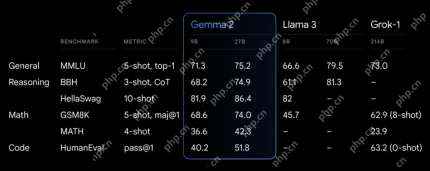 Exploring the Capabilities of Google's Gemma 2 ModelsApr 22, 2025 am 11:26 AM
Google's Gemma 2: A Powerful, Efficient Language Model Google's Gemma family of language models, celebrated for efficiency and performance, has expanded with the arrival of Gemma 2. This latest release comprises two models: a 27-billion parameter ver
 The Next Wave of GenAI: Perspectives with Dr. Kirk Borne - Analytics VidhyaApr 22, 2025 am 11:21 AM
This Leading with Data episode features Dr. Kirk Borne, a leading data scientist, astrophysicist, and TEDx speaker. A renowned expert in big data, AI, and machine learning, Dr. Borne offers invaluable insights into the current state and future traje
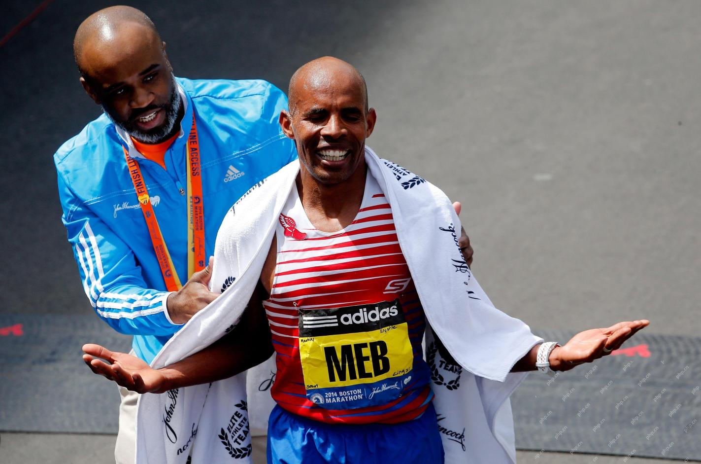 AI For Runners And Athletes: We're Making Excellent ProgressApr 22, 2025 am 11:12 AM
There were some very insightful perspectives in this speech—background information about engineering that showed us why artificial intelligence is so good at supporting people’s physical exercise. I will outline a core idea from each contributor’s perspective to demonstrate three design aspects that are an important part of our exploration of the application of artificial intelligence in sports. Edge devices and raw personal data This idea about artificial intelligence actually contains two components—one related to where we place large language models and the other is related to the differences between our human language and the language that our vital signs “express” when measured in real time. Alexander Amini knows a lot about running and tennis, but he still
 Jamie Engstrom On Technology, Talent And Transformation At CaterpillarApr 22, 2025 am 11:10 AM
Caterpillar's Chief Information Officer and Senior Vice President of IT, Jamie Engstrom, leads a global team of over 2,200 IT professionals across 28 countries. With 26 years at Caterpillar, including four and a half years in her current role, Engst
 New Google Photos Update Makes Any Photo Pop With Ultra HDR QualityApr 22, 2025 am 11:09 AM
Google Photos' New Ultra HDR Tool: A Quick Guide Enhance your photos with Google Photos' new Ultra HDR tool, transforming standard images into vibrant, high-dynamic-range masterpieces. Ideal for social media, this tool boosts the impact of any photo,


Hot AI Tools

Undresser.AI Undress
AI-powered app for creating realistic nude photos

AI Clothes Remover
Online AI tool for removing clothes from photos.

Undress AI Tool
Undress images for free

Clothoff.io
AI clothes remover

Video Face Swap
Swap faces in any video effortlessly with our completely free AI face swap tool!

Hot Article
Hot Tools

Atom editor mac version download
The most popular open source editor

SublimeText3 Linux new version
SublimeText3 Linux latest version

mPDF
mPDF is a PHP library that can generate PDF files from UTF-8 encoded HTML. The original author, Ian Back, wrote mPDF to output PDF files "on the fly" from his website and handle different languages. It is slower than original scripts like HTML2FPDF and produces larger files when using Unicode fonts, but supports CSS styles etc. and has a lot of enhancements. Supports almost all languages, including RTL (Arabic and Hebrew) and CJK (Chinese, Japanese and Korean). Supports nested block-level elements (such as P, DIV),

Zend Studio 13.0.1
Powerful PHP integrated development environment

SecLists
SecLists is the ultimate security tester's companion. It is a collection of various types of lists that are frequently used during security assessments, all in one place. SecLists helps make security testing more efficient and productive by conveniently providing all the lists a security tester might need. List types include usernames, passwords, URLs, fuzzing payloads, sensitive data patterns, web shells, and more. The tester can simply pull this repository onto a new test machine and he will have access to every type of list he needs.

