More versatile and effective, Ant’s self-developed optimizer WSAM was selected into KDD Oral

The generalization ability of deep neural networks (DNNs) is closely related to the flatness of the extreme points, so the Sharpness-Aware Minimization (SAM) algorithm has emerged to find flatter extreme points to improve the generalization ability. . This paper re-examines the loss function of SAM and proposes a more general and effective method, WSAM, to improve the flatness of training extreme points by using flatness as a regularization term. Experiments on various public datasets show that compared with the original optimizer, SAM and its variants, WSAM achieves better generalization performance in the vast majority of cases. WSAM has also been widely adopted in Ant's internal digital payment, digital finance and other scenarios and has achieved remarkable results. This paper was accepted as an Oral Paper by KDD '23.

• ##Paper address: https: //arxiv.org/pdf/2305.15817.pdf
• Code address: https://github.com/intelligent-machine-learning/dlrover/tree/ master/atorch/atorch/optimizers

#With the development of deep learning technology, highly over-parameterized DNNs are used in various machine learning scenarios such as CV and NLP. It was a huge success. Although over-parameterized models tend to overfit the training data, they usually have good generalization capabilities. The secret of generalization has attracted more and more attention and has become a popular research topic in the field of deep learning.

The latest research shows that generalization ability is closely related to the flatness of extreme points. In other words, the presence of flat extreme points in the "landscape" of the loss function allows for smaller generalization errors. Sharpness-Aware Minimization (SAM) [1] is a technique for finding flatter extreme points and is considered to be one of the most promising technical directions currently. SAM technology is widely used in many fields such as computer vision, natural language processing, and two-layer learning, and significantly outperforms previous state-of-the-art methods in these fields

In order to explore a flatter The minimum value of , SAM defines the flatness of the loss function L at w as follows:

GSAM [2] proved is an approximation of the maximum eigenvalue of the Hessian matrix at the local extreme point, indicating that is indeed an effective measure of flatness (steepness). However can only be used to find flatter areas rather than minimum points, which may cause the loss function to converge to a point where the loss value is still large (although the surrounding area is flat). Therefore, SAM uses , that is, as the loss function. It can be seen as a compromise between finding a flatter surface and smaller loss value between and , where both are given equal weight.

This article rethinks the construction of and regards as a regularization term. We have developed a more general and effective algorithm called WSAM (Weighted Sharpness-Aware Minimization), whose loss function adds a weighted flatness term as a regular term, in which the hyperparameter Controls the weight of flatness. In the method introduction chapter, we demonstrated how to use to guide the loss function to find flatter or smaller extreme points. Our key contributions can be summarized as follows.

• We propose WSAM, which treats flatness as a regularization term and gives different weights between different tasks. We propose a "weight decoupling" technique to handle the regularization term in the update formula, aiming to accurately reflect the flatness of the current step. When the underlying optimizer is not SGD, such as SGDM and Adam, WSAM differs significantly from SAM in form. Ablation experiments show that this technique improves performance in most cases.
• We verified the effectiveness of WSAM on common tasks on public datasets. Experimental results show that compared with SAM and its variants, WSAM has better generalization performance in most situations.

Preliminary knowledge

SAM is to solve the minimax optimization problem of defined by formula (1) a technology.

First, SAM uses the first-order Taylor expansion around w to approximate the maximization problem of the inner layer, that is, ,

##Secondly, SAM updates w by adopting the approximate gradient of , i.e.

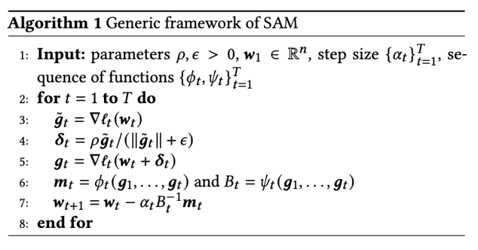
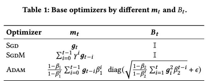
The second approximation is for acceleration calculate. Other gradient-based optimizers (called base optimizers) can be incorporated into the general framework of SAM, see Algorithm 1 for details. By changing and in Algorithm 1, we can get different basic optimizers, such as SGD, SGDM and Adam, see Tab. 1. Note that Algorithm 1 falls back to the original SAM from the SAM paper [1] when the base optimizer is SGD.

##Method introduction

Design details of WSAM

Here, we give the formal definition of

, which consists of a regular loss and a flatness term. From formula (1), we have

in . When =0, degenerates into a regular loss; when =1/2, is equivalent to ; When >1/2, pays more attention to flatness, so it is easier to find points with smaller curvature rather than smaller loss values ​​compared with SAM; vice versa; Likewise.

A general framework for WSAM that includes different base optimizers can be implemented by choosing different and , see Algorithm 2. For example, when and , we get WSAM whose base optimizer is SGD, see Algorithm 3. Here, we adopt a "weight decoupling" technique, that is, the flatness term is not integrated with the base optimizer for calculating gradients and updating weights, but is calculated independently (the last term on line 7 of Algorithm 2 ). In this way, the effect of regularization only reflects the flatness of the current step without additional information. For comparison, Algorithm 4 gives a WSAM without "weight decoupling" (called Coupled-WSAM). For example, if the underlying optimizer is SGDM, the regularization term of Coupled-WSAM is an exponential moving average of flatness. As shown in the experimental section, "weight decoupling" can improve generalization performance in most cases.

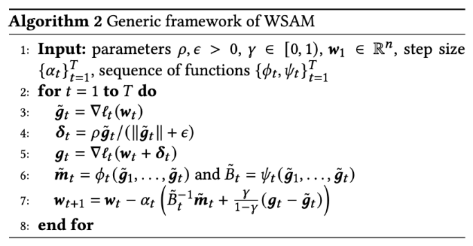
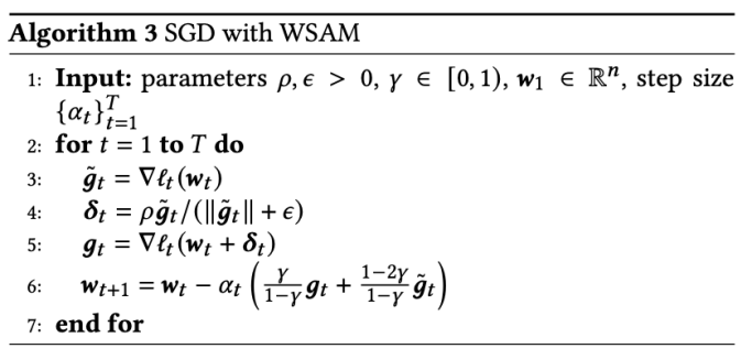
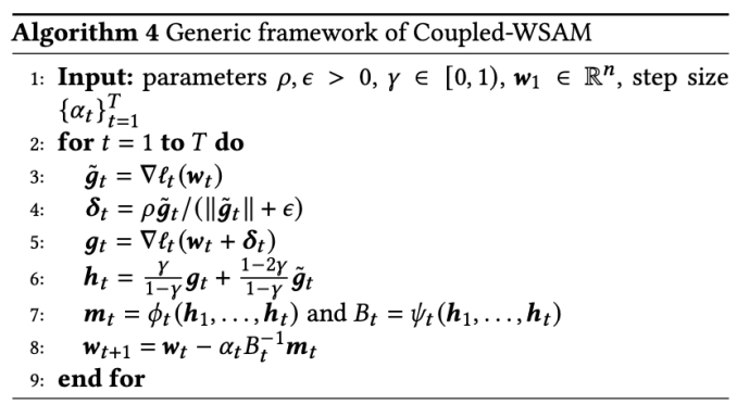
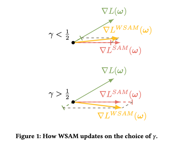
Fig. 1 shows the WSAM update process under different values. When , is between and , and As increases, it gradually deviates from .

Simple example

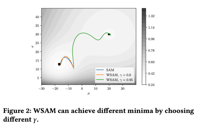
In order to better illustrate the effect and advantages of γ in WSAM, we set Here is a simple two-dimensional example. As shown in Fig. 2, the loss function has a relatively uneven extreme point in the lower left corner (position: (-16.8, 12.8), loss value: 0.28), and a flat extreme point in the upper right corner (position: (19.8, 29.9), loss value: 0.36). The loss function is defined as: , where is the KL divergence between the univariate Gaussian model and two normal distributions, that is, , where and .

We use SGDM with a momentum of 0.9 as the base optimizer and set =2 for SAM and WSAM. Starting from the initial point (-6, 10), the loss function is optimized in 150 steps using a learning rate of 5. SAM converges to the extreme point where the loss value is lower but more uneven, and the WSAM of =0.6 is similar. However, =0.95 causes the loss function to converge to a flat extreme point, indicating that stronger flatness regularization plays a role.

Experiments

We conducted experiments on various tasks to verify the effectiveness of WSAM .

Image Classification

We first studied the effect of WSAM on training models from scratch on the Cifar10 and Cifar100 datasets. The models we selected include ResNet18 and WideResNet-28-10. We train models on Cifar10 and Cifar100 using predefined batch sizes of 128, 256 for ResNet18 and WideResNet-28-10 respectively. The base optimizer used here is SGDM with momentum 0.9. According to the settings of SAM [1], each basic optimizer runs twice the number of epochs as the SAM class optimizer. We trained both models for 400 epochs (200 epochs for the SAM class optimizer) and used a cosine scheduler to decay the learning rate. Here we do not use other advanced data augmentation methods such as cutout and AutoAugment.

For both models, we use joint grid search to determine the learning rate and weight decay coefficients of the base optimizer and keep them constant for the following SAM-like optimizer experiments. The search ranges of learning rate and weight decay coefficient are {0.05, 0.1} and {1e-4, 5e-4, 1e-3} respectively. Since all SAM class optimizers have a hyperparameter (neighborhood size), we next search for the best on the SAM optimizer and use the same value for other SAMs Class optimizer. The search range of is {0.01, 0.02, 0.05, 0.1, 0.2, 0.5}. Finally, we searched for the unique hyperparameters of other SAM class optimizers, and the search range came from the recommended range of their respective original articles. For GSAM [2], we search in the range {0.01, 0.02, 0.03, 0.1, 0.2, 0.3}. For ESAM [3], we search for in the range {0.4, 0.5, 0.6}, within the range {0.4, 0.5, 0.6}, and Search within the range {0.4, 0.5, 0.6}. 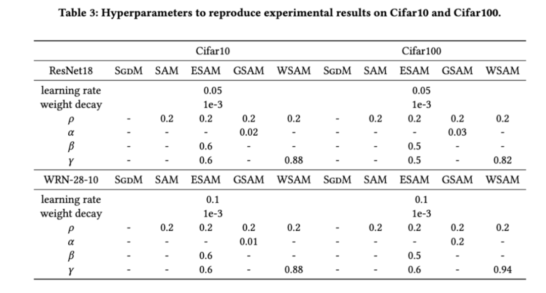For WSAM, we search for in the range {0.5, 0.6, 0.7, 0.8, 0.82, 0.84, 0.86, 0.88, 0.9, 0.92, 0.94, 0.96}. We repeated the experiment 5 times using different random seeds and calculated the mean error and standard deviation. We conduct experiments on a single-card NVIDIA A100 GPU. Optimizer hyperparameters for each model are summarized in Tab. 3.

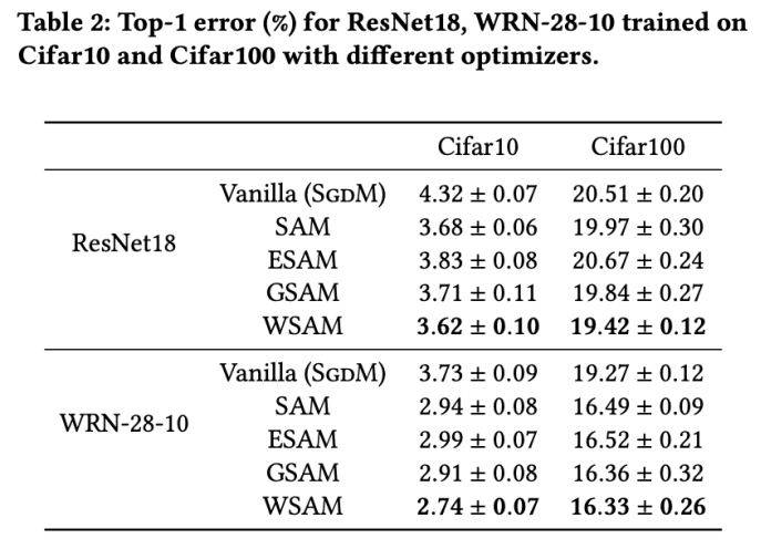
Tab. 2 shows the top-test results of ResNet18 and WRN-28-10 on Cifar10 and Cifar100 under different optimizers. 1 error rate. Compared with the basic optimizer, the SAM class optimizer significantly improves the performance. At the same time, WSAM is significantly better than other SAM class optimizers.

Additional training on ImageNet

We further use Data-Efficient Image on the ImageNet dataset Transformers network structure for experiments. We resume a pre-trained DeiT-base checkpoint and then continue training for three epochs. The model is trained using a batch size of 256, the base optimizer is SGDM with momentum 0.9, the weight decay coefficient is 1e-4, and the learning rate is 1e-5. We repeated the run 5 times on a four-card NVIDIA A100 GPU and calculated the average error and standard deviation

We searched for SAM in {0.05, 0.1, 0.5, 1.0,⋯ , 6.0} the best of. The optimal =5.5 is used directly for other SAM class optimizers. After that, we search for the best of GSAM in {0.01, 0.02, 0.03, 0.1, 0.2, 0.3} and the best of WSAM between 0.80 and 0.98 with a step size of 0.02 .

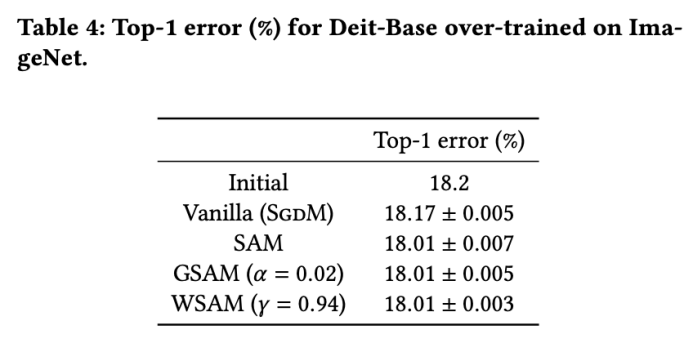
The initial top-1 error rate of the model is 18.2%, and after three additional epochs, the error rate is shown in Tab. 4. We do not find significant differences between the three SAM-like optimizers, but they all outperform the base optimizer, indicating that they can find flatter extreme points and have better generalization capabilities.

Robustness to label noise

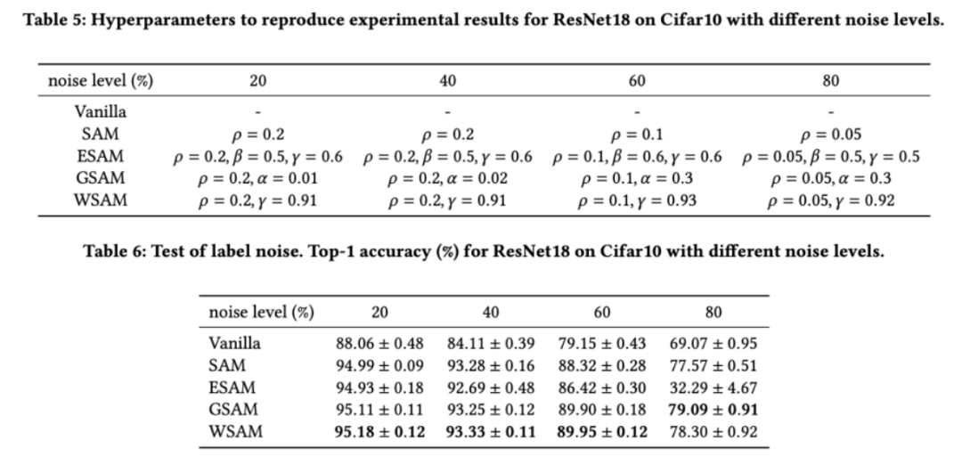
As shown in previous studies [1, 4, 5], SAM class optimizers perform well in the presence of label noise in the training set Produces good robustness. Here, we compare the robustness of WSAM with SAM, ESAM, and GSAM. We train ResNet18 on the Cifar10 dataset for 200 epochs and inject symmetric label noise with noise levels of 20%, 40%, 60% and 80%. We use SGDM with 0.9 momentum as the base optimizer, a batch size of 128, a learning rate of 0.05, a weight decay coefficient of 1e-3, and a cosine scheduler to decay the learning rate. For each label noise level, we performed a grid search on the SAM within the range {0.01, 0.02, 0.05, 0.1, 0.2, 0.5} to determine a common value. We then individually search for other optimizer-specific hyperparameters to find optimal generalization performance. We list the hyperparameters required to reproduce our results in Tab. 5. We present the results of the robustness test in Tab. 6. WSAM generally has better robustness than SAM, ESAM and GSAM.

Exploring the impact of geometric structures

The SAM class optimizer can be used with ASAM [4] and Fisher Techniques such as SAM [5] are combined to adaptively adjust the shape of the explored neighborhood. We conduct experiments on WRN-28-10 on Cifar10 to compare the performance of SAM and WSAM when using adaptive and Fisher information methods, respectively, to understand how the geometry of the exploration region affects the generalization performance of SAM-like optimizers.

Except for the parameters except and , we reuse the configuration in image classification. According to previous studies [4, 5], the of ASAM and Fisher SAM are usually larger. We search for the best in {0.1, 0.5, 1.0,…, 6.0}, and the best for both ASAM and Fisher SAM is 5.0. After that, we searched for the best of WSAM between 0.80 and 0.94 with a step size of 0.02, and the best of both methods was 0.88.

Surprisingly, as shown in Tab. 7, the baseline WSAM shows better generalization even among multiple candidates. Therefore, we recommend directly using WSAM with a fixed baseline.

Ablation Experiment

In this section, we conduct ablation experiments to gain a deeper understanding of WSAM The importance of "weight decoupling" technology. As described in the design details of WSAM, we compare the WSAM variant without "weight decoupling" (Algorithm 4) Coupled-WSAM with the original method.

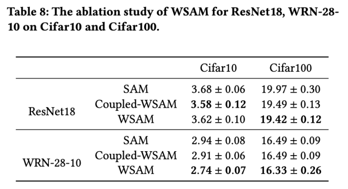
The results are shown in Tab. 8. Coupled-WSAM produces better results than SAM in most cases, and WSAM further improves the results in most cases, demonstrating the effectiveness of the "weight decoupling" technique.

Extreme point analysis

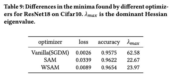
Here, we further deepen our understanding of the WSAM optimizer by comparing the differences between the extreme points found by the WSAM and SAM optimizers. understand. The flatness (steepness) at extreme points can be described by the maximum eigenvalue of the Hessian matrix. The larger the eigenvalue, the less flat it is. We use the Power Iteration algorithm to calculate this maximum eigenvalue.

Tab. 9 shows the difference between the extreme points found by the SAM and WSAM optimizers. We find that the extreme points found by the vanilla optimizer have smaller loss values ​​but are less flat, while the extreme points found by SAM have larger loss values ​​but are flatter, thus improving generalization performance. Interestingly, the extreme points found by WSAM not only have much smaller loss values ​​than SAM, but also have a flatness that is very close to SAM. This shows that in the process of finding extreme points, WSAM prioritizes ensuring smaller loss values ​​while trying to search for flatter areas.

Hyperparameter sensitivity

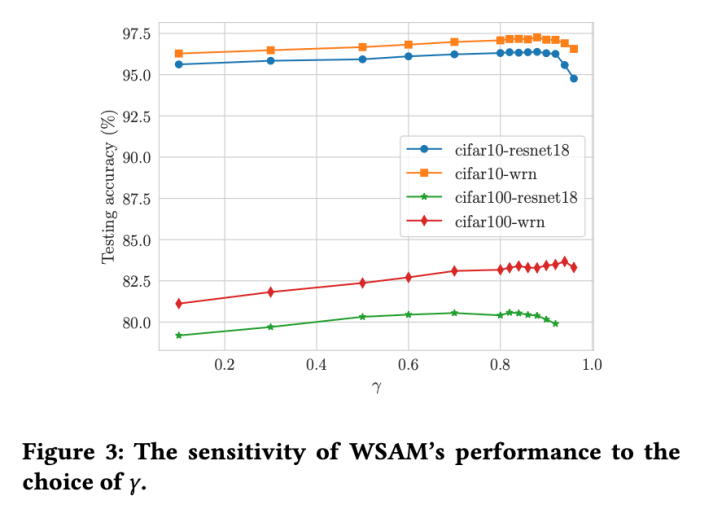
Compared with SAM, WSAM has an additional hyperparameter, used to scale the size of the flat (steep) degree term. Here, we test the sensitivity of WSAM's generalization performance to this hyperparameter. We trained ResNet18 and WRN-28-10 models using WSAM on Cifar10 and Cifar100, using a wide range of values. As shown in Fig. 3, the results show that WSAM is not sensitive to the choice of hyperparameters. We also found that the optimal generalization performance of WSAM is almost always between 0.8 and 0.95.

The above is the detailed content of More versatile and effective, Ant’s self-developed optimizer WSAM was selected into KDD Oral. For more information, please follow other related articles on the PHP Chinese website!