How to implement gradient descent to solve logistic regression in python

Linear regression

1. Linear regression function

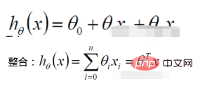
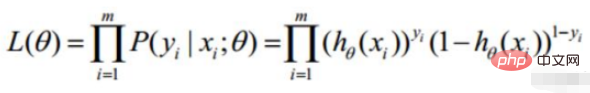
Definition of likelihood function: given joint sample valueXThe following functions about (unknown) parameters

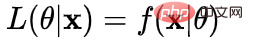
##Likelihood function: What Such parameters are exactly the true values ​​when combined with our data.

2. Linear regression likelihood function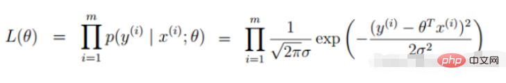

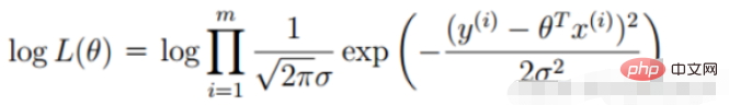
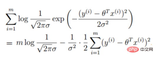
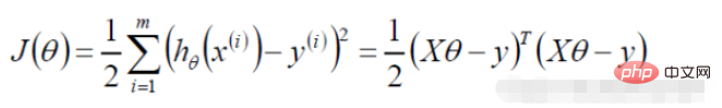
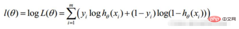
Log likelihood:

3. Linear regression objective function

(expression of error, our purpose is to make the difference between the true value and the predicted value Minimum error)

(The derivative is 0 to obtain the extreme value, and the parameters of the function are obtained)

Logistic regression

Logistic regression is linear The regression result is added with a layer of Sigmoid function

1. Logistic regression function

2. Logistic regression likelihood function

Premise data obeys Bernoulli distribution

Log likelihood:

Introduction

Convert to gradient descent task, logistic regression objective function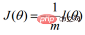

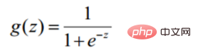
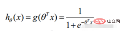
Gradient descent method solution

My understanding is to seek derivation and update parameters, stop after reaching a certain condition, and obtain an approximately optimal solution

Code implementation

Sigmoid function

def sigmoid(z):    
   return 1 / (1 + np.exp(-z))

Prediction function

def model(X, theta):    
    return sigmoid(np.dot(X, theta.T))

Objective function

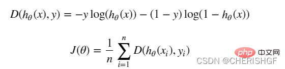
def cost(X, y, theta):    
     left = np.multiply(-y, np.log(model(X, theta)))    
     right = np.multiply(1 - y, np.log(1 - model(X, theta)))    
     return np.sum(left - right) / (len(X))

Gradient

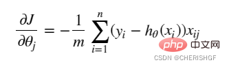
def gradient(X, y, theta):    
  grad = np.zeros(theta.shape)    
  error = (model(X, theta)- y).ravel()    
  for j in range(len(theta.ravel())): #for each parmeter        
     term = np.multiply(error, X[:,j])        
     grad[0, j] = np.sum(term) / len(X)    
   return grad

Gradient descent stopping strategy

STOP_ITER = 0
STOP_COST = 1
STOP_GRAD = 2
 
def stopCriterion(type, value, threshold):
    # 设定三种不同的停止策略
    if type == STOP_ITER:  # 设定迭代次数
        return value > threshold
    elif type == STOP_COST:  # 根据损失值停止
        return abs(value[-1] - value[-2]) < threshold
    elif type == STOP_GRAD:  # 根据梯度变化停止
        return np.linalg.norm(value) < threshold

Sample reshuffle

import numpy.random
#洗牌
def shuffleData(data):
    np.random.shuffle(data)
    cols = data.shape[1]
    X = data[:, 0:cols-1]
    y = data[:, cols-1:]
    return X, y

Gradient descent solution

def descent(data, theta, batchSize, stopType, thresh, alpha):
    # 梯度下降求解
 
    init_time = time.time()
    i = 0  # 迭代次数
    k = 0  # batch
    X, y = shuffleData(data)
    grad = np.zeros(theta.shape)  # 计算的梯度
    costs = [cost(X, y, theta)]  # 损失值
 
    while True:
        grad = gradient(X[k:k + batchSize], y[k:k + batchSize], theta)
        k += batchSize  # 取batch数量个数据
        if k >= n:
            k = 0
            X, y = shuffleData(data)  # 重新洗牌
        theta = theta - alpha * grad  # 参数更新
        costs.append(cost(X, y, theta))  # 计算新的损失
        i += 1
 
        if stopType == STOP_ITER:
            value = i
        elif stopType == STOP_COST:
            value = costs
        elif stopType == STOP_GRAD:
            value = grad
        if stopCriterion(stopType, value, thresh): break
 
    return theta, i - 1, costs, grad, time.time() - init_time

Complete code

import numpy as np
import pandas as pd
import matplotlib.pyplot as plt
import os
import numpy.random
import time
 
 
def sigmoid(z):
    return 1 / (1 + np.exp(-z))
 
 
def model(X, theta):
    return sigmoid(np.dot(X, theta.T))
 
 
def cost(X, y, theta):
    left = np.multiply(-y, np.log(model(X, theta)))
    right = np.multiply(1 - y, np.log(1 - model(X, theta)))
    return np.sum(left - right) / (len(X))
 
 
def gradient(X, y, theta):
    grad = np.zeros(theta.shape)
    error = (model(X, theta) - y).ravel()
    for j in range(len(theta.ravel())):  # for each parmeter
        term = np.multiply(error, X[:, j])
        grad[0, j] = np.sum(term) / len(X)
    return grad
 
 
STOP_ITER = 0
STOP_COST = 1
STOP_GRAD = 2
 
 
def stopCriterion(type, value, threshold):
    # 设定三种不同的停止策略
    if type == STOP_ITER:  # 设定迭代次数
        return value > threshold
    elif type == STOP_COST:  # 根据损失值停止
        return abs(value[-1] - value[-2]) < threshold
    elif type == STOP_GRAD:  # 根据梯度变化停止
        return np.linalg.norm(value) < threshold
 
 
# 洗牌
def shuffleData(data):
    np.random.shuffle(data)
    cols = data.shape[1]
    X = data[:, 0:cols - 1]
    y = data[:, cols - 1:]
    return X, y
 
 
def descent(data, theta, batchSize, stopType, thresh, alpha):
    # 梯度下降求解
 
    init_time = time.time()
    i = 0  # 迭代次数
    k = 0  # batch
    X, y = shuffleData(data)
    grad = np.zeros(theta.shape)  # 计算的梯度
    costs = [cost(X, y, theta)]  # 损失值
 
    while True:
        grad = gradient(X[k:k + batchSize], y[k:k + batchSize], theta)
        k += batchSize  # 取batch数量个数据
        if k >= n:
            k = 0
            X, y = shuffleData(data)  # 重新洗牌
        theta = theta - alpha * grad  # 参数更新
        costs.append(cost(X, y, theta))  # 计算新的损失
        i += 1
 
        if stopType == STOP_ITER:
            value = i
        elif stopType == STOP_COST:
            value = costs
        elif stopType == STOP_GRAD:
            value = grad
        if stopCriterion(stopType, value, thresh): break
 
    return theta, i - 1, costs, grad, time.time() - init_time
 
 
def runExpe(data, theta, batchSize, stopType, thresh, alpha):
    # import pdb
    # pdb.set_trace()
    theta, iter, costs, grad, dur = descent(data, theta, batchSize, stopType, thresh, alpha)
    name = "Original" if (data[:, 1] > 2).sum() > 1 else "Scaled"
    name += " data - learning rate: {} - ".format(alpha)
    if batchSize == n:
        strDescType = "Gradient"  # 批量梯度下降
    elif batchSize == 1:
        strDescType = "Stochastic"  # 随机梯度下降
    else:
        strDescType = "Mini-batch ({})".format(batchSize)  # 小批量梯度下降
    name += strDescType + " descent - Stop: "
    if stopType == STOP_ITER:
        strStop = "{} iterations".format(thresh)
    elif stopType == STOP_COST:
        strStop = "costs change < {}".format(thresh)
    else:
        strStop = "gradient norm < {}".format(thresh)
    name += strStop
    print("***{}\nTheta: {} - Iter: {} - Last cost: {:03.2f} - Duration: {:03.2f}s".format(
        name, theta, iter, costs[-1], dur))
    fig, ax = plt.subplots(figsize=(12, 4))
    ax.plot(np.arange(len(costs)), costs, 'r')
    ax.set_xlabel('Iterations')
    ax.set_ylabel('Cost')
    ax.set_title(name.upper() + ' - Error vs. Iteration')
    return theta
 
 
path = 'data' + os.sep + 'LogiReg_data.txt'
pdData = pd.read_csv(path, header=None, names=['Exam 1', 'Exam 2', 'Admitted'])
positive = pdData[pdData['Admitted'] == 1]
negative = pdData[pdData['Admitted'] == 0]
 
# 画图观察样本情况
fig, ax = plt.subplots(figsize=(10, 5))
ax.scatter(positive['Exam 1'], positive['Exam 2'], s=30, c='b', marker='o', label='Admitted')
ax.scatter(negative['Exam 1'], negative['Exam 2'], s=30, c='r', marker='x', label='Not Admitted')
ax.legend()
ax.set_xlabel('Exam 1 Score')
ax.set_ylabel('Exam 2 Score')
 
pdData.insert(0, 'Ones', 1)
 
# 划分训练数据与标签
orig_data = pdData.values
cols = orig_data.shape[1]
X = orig_data[:, 0:cols - 1]
y = orig_data[:, cols - 1:cols]
# 设置初始参数0
theta = np.zeros([1, 3])
 
# 选择的梯度下降方法是基于所有样本的
n = 100
runExpe(orig_data, theta, n, STOP_ITER, thresh=5000, alpha=0.000001)
runExpe(orig_data, theta, n, STOP_COST, thresh=0.000001, alpha=0.001)
runExpe(orig_data, theta, n, STOP_GRAD, thresh=0.05, alpha=0.001)
runExpe(orig_data, theta, 1, STOP_ITER, thresh=5000, alpha=0.001)
runExpe(orig_data, theta, 1, STOP_ITER, thresh=15000, alpha=0.000002)
runExpe(orig_data, theta, 16, STOP_ITER, thresh=15000, alpha=0.001)
 
from sklearn import preprocessing as pp
 
# 数据预处理
scaled_data = orig_data.copy()
scaled_data[:, 1:3] = pp.scale(orig_data[:, 1:3])
 
runExpe(scaled_data, theta, n, STOP_ITER, thresh=5000, alpha=0.001)
runExpe(scaled_data, theta, n, STOP_GRAD, thresh=0.02, alpha=0.001)
theta = runExpe(scaled_data, theta, 1, STOP_GRAD, thresh=0.002 / 5, alpha=0.001)
runExpe(scaled_data, theta, 16, STOP_GRAD, thresh=0.002 * 2, alpha=0.001)
 
 
# 设定阈值
def predict(X, theta):
    return [1 if x >= 0.5 else 0 for x in model(X, theta)]
 
 
# 计算精度
scaled_X = scaled_data[:, :3]
y = scaled_data[:, 3]
predictions = predict(scaled_X, theta)
correct = [1 if ((a == 1 and b == 1) or (a == 0 and b == 0)) else 0 for (a, b) in zip(predictions, y)]
accuracy = (sum(map(int, correct)) % len(correct))
print('accuracy = {0}%'.format(accuracy))

Advantages and disadvantages of logistic regression

Advantages

• The form is simple and the interpretability of the model is very good. From the weight of the feature, we can see the impact of different features on the final result. If the weight value of a certain feature is relatively high, then this feature will have a greater impact on the final result.

• The model works well. It is acceptable in engineering (as a baseline). If feature engineering is done well, the effect will not be too bad, and feature engineering can be developed in parallel, greatly speeding up development.

• Training speed is faster. When classifying, the amount of calculation is only related to the number of features. Moreover, the distributed optimization sgd of logistic regression is relatively mature, and the training speed can be further improved through heap machines, so that we can iterate several versions of the model in a short period of time.

• It takes up little resources, especially memory. Because only the feature values ​​of each dimension need to be stored.

• Conveniently adjust the output results. Logistic regression can easily obtain the final classification result, because the output is the probability score of each sample, and we can easily cutoff these probability scores, that is, divide the threshold (those greater than a certain threshold are classified into one category, and those less than a certain threshold are classified into one category). A certain threshold is a category).

Disadvantages

• The accuracy is not very high. Because the form is very simple (very similar to a linear model), it is difficult to fit the true distribution of the data.

• It is difficult to deal with the problem of data imbalance. For example: If we deal with a problem where positive and negative samples are very unbalanced, such as the ratio of positive and negative samples is 10000:1. If we predict all samples as positive, we can also make the value of the loss function smaller. But as a classifier, its ability to distinguish positive and negative samples will not be very good.

• Processing nonlinear data is more troublesome. Logistic regression, without introducing other methods, can only handle linearly separable data, or further, handle binary classification problems.

• Logistic regression itself cannot filter features. Sometimes, we use gbdt to filter features and then use logistic regression.

The above is the detailed content of How to implement gradient descent to solve logistic regression in python. For more information, please follow other related articles on the PHP Chinese website!