How to use NumPy in Python common functions

1. txt file

(1) Identity matrix

is a square matrix in which the elements on the main diagonal are all 1 and the remaining elements are 0 .

In NumPy, you can use the eye function to create such a two-dimensional array. We only need to give a parameter to specify the number of 1 elements in the matrix.

For example, create an array of 3×3:

import numpy as np
I2 = np.eye(3)
print(I2)
[[1. 0. 0.]
 [0. 1. 0.]
 [0. 0. 1.]]

(2) Use the savetxt function to store data into a file. Of course, we need to specify the file name and the array to be saved.

np.savetxt('eye.txt', I2)#创建一个eye.txt文件，用于保存I2的数据

2. CSV file

CSV (Comma-Separated Value) format is a common file format; usually, the database dump file It is in CSV format, and each field in the file corresponds to the column in the database table; spreadsheet software (such as Microsoft Excel) can process CSV files.

note: The loadtxt function in NumPy can easily read CSV files, automatically segment fields, and load data into NumPy arrays

Data content of data.csv:

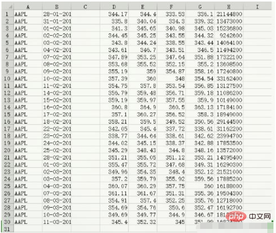
c, v = np.loadtxt('data.csv', delimiter=',', usecols=(6,7), unpack=True)
# usecols的参数为一个元组，以获取第7字段至第8字段的数据
# unpack参数设置为True，意思是分拆存储不同列的数据，即分别将收盘价和成交量的数组赋值给变量c和v
print(c)
[336.1  339.32 345.03 344.32 343.44 346.5  351.88 355.2  358.16 354.54
 356.85 359.18 359.9  363.13 358.3  350.56 338.61 342.62 342.88 348.16
 353.21 349.31 352.12 359.56 360.   355.36 355.76 352.47 346.67 351.99]
print(v)
[21144800. 13473000. 15236800.  9242600. 14064100. 11494200. 17322100.
 13608500. 17240800. 33162400. 13127500. 11086200. 10149000. 17184100.
 18949000. 29144500. 31162200. 23994700. 17853500. 13572000. 14395400.
 16290300. 21521000. 17885200. 16188000. 19504300. 12718000. 16192700.
 18138800. 16824200.]
print(type(c))
print(type(v))
<class &#39;numpy.ndarray&#39;>
<class &#39;numpy.ndarray&#39;>

3.Volume Weighted Average Price = average() function

VWAP Overview: VWAP(Volume- Weighted Average Price (Volume Weighted Average Price) is a very important economic quantity, which represents the "average" price of financial assets.

The higher the trading volume of a certain price, the greater the weight of that price.

VWAP is a weighted average calculated with trading volume as the weight, and is often used in algorithmic trading.

vwap = np.average(c,weights=v)
print('成交量加权平均价格vwap =', vwap)
成交量加权平均价格vwap = 350.5895493532009

4. Arithmetic mean function = mean() function

The mean function in NumPy can calculate the arithmetic mean of array elements

print('c数组中元素的算数平均值为： {}'.format(np.mean(c)))
c数组中元素的算数平均值为： 351.0376666666667

5. Time-Weighted Average Price

Overview of TWAP:

In economics, TWAP (Time-Weighted Average Price, time-weighted average price) is another " Average price indicator. Now that we have calculated VWAP, let’s calculate TWAP as well. In fact, TWAP is just a variant. The basic idea is that the recent price is more important, so we should give a higher weight to the recent price. The simplest method is to use the arange function to create a sequence of natural numbers that starts from 0 and increases sequentially. The number of natural numbers is the number of closing prices. Of course, this is not necessarily the correct way to calculate TWAP.

t = np.arange(len(c))
print('时间加权平均价格twap=', np.average(c, weights=t))
时间加权平均价格twap= 352.4283218390804

6. Maximum and minimum values

h, l = np.loadtxt('data.csv', delimiter=',', usecols=(4,5), unpack=True)
print('h数据为： \n{}'.format(h))
print('-'*10)
print('l数据为： \n{}'.format(l))
h数据为： 
[344.4  340.04 345.65 345.25 344.24 346.7  353.25 355.52 359.   360.
 357.8  359.48 359.97 364.9  360.27 359.5  345.4  344.64 345.15 348.43
 355.05 355.72 354.35 359.79 360.29 361.67 357.4  354.76 349.77 352.32]
----------
l数据为： 
[333.53 334.3  340.98 343.55 338.55 343.51 347.64 352.15 354.87 348.
 353.54 356.71 357.55 360.5  356.52 349.52 337.72 338.61 338.37 344.8
 351.12 347.68 348.4  355.92 357.75 351.31 352.25 350.6  344.9  345.  ]
print('h数据的最大值为： {}'.format(np.max(h)))
print('l数据的最小值为： {}'.format(np.min(l)))
h数据的最大值为： 364.9
l数据的最小值为： 333.53
NumPy中有一个ptp函数可以计算数组的取值范围
该函数返回的是数组元素的最大值和最小值之间的差值
也就是说，返回值等于max(array) - min(array)
print('h数据的最大值-最小值的差值为： \n{}'.format(np.ptp(h)))
print('l数据的最大值-最小值的差值为： \n{}'.format(np.ptp(l)))
h数据的最大值-最小值的差值为： 
24.859999999999957
l数据的最大值-最小值的差值为： 
26.970000000000027

7. Statistical analysis

Median: We can use Some thresholds are used to remove outliers, but there is a better way, which is the median.

Arrange the variable values ​​in order of size to form a sequence. The number in the middle of the sequence is the median.

For example, if we have 5 values ​​​​1, 2, 3, 4, and 5, then the median is the middle number 3.

m = np.loadtxt('data.csv', delimiter=',', usecols=(6,), unpack=True)
print('m数据中的中位数为： {}'.format(np.median(m)))
m数据中的中位数为： 352.055
# 数组排序后，查找中位数
sorted_m = np.msort(m)
print('m数据排序： \n{}'.format(sorted_m))
N = len(c)
print('m数据中的中位数为： {}'.format((sorted_m[N//2]+sorted_m[(N-1)//2])/2))
m数据排序： 
[336.1  338.61 339.32 342.62 342.88 343.44 344.32 345.03 346.5  346.67
 348.16 349.31 350.56 351.88 351.99 352.12 352.47 353.21 354.54 355.2
 355.36 355.76 356.85 358.16 358.3  359.18 359.56 359.9  360.   363.13]
m数据中的中位数为： 352.055
方差：
方差是指各个数据与所有数据算术平均数的离差平方和除以数据个数所得到的值。
print('variance =', np.var(m))
variance = 50.126517888888884
var_hand = np.mean((m-m.mean())**2)
print('var =', var_hand)
var = 50.126517888888884

Note: The difference in calculation between sample variance and population variance. The population variance is the sum of squares of deviations divided by the number of data, while the sample variance is the sum of squares of deviations divided by the number of sample data minus 1, where the number of sample data minus 1 (i.e. n-1) is called the degree of freedom. The reason for this difference is to ensure that the sample variance is an unbiased estimator.

8. Stock Return

In academic literature, the analysis of closing prices is often based on stock returns and logarithmic returns.

The simple rate of return refers to the rate of change between two adjacent prices, while the logarithmic rate of return refers to the difference between the two after taking the logarithm of all prices.
We learned about logarithms in high school. The logarithm of "a" minus the logarithm of "b" is equal to the logarithm of "a divided by b". Therefore, the log return can also be used to measure the rate of change of price.

Note that since the rate of return is a ratio, for example, we divide US dollars by US dollars (it can also be other currency units), it is dimensionless.

In short, what investors are most interested in is the variance or standard deviation of the rate of return, because it represents the size of the investment risk.

(1) First, let’s calculate the simple rate of return. The diff function in NumPy can return an array consisting of the difference between adjacent array elements. This is somewhat similar to differential calculus. To calculate the yield, we also need to divide the previous day's price by the difference. However, please note here that the array returned by diff has one element less than the closing price array. returns = np.diff(arr)/arr[:-1]

Note that we do not use the last value in the closing price array as the divisor. Next, use the std function to calculate the standard deviation:

print ("Standard deviation =", np.std(returns))

(2) The logarithmic return is even simpler to calculate. We first use the log function to get the logarithm of each closing price, and then use the diff function on the result.

logreturns = np.diff( np.log(c) )

Generally, we should check the input array to ensure that it does not contain zeros and negative numbers. Otherwise, you will get an error message. However, in our example, the stock price is always positive, so the check can be omitted.

(3) We are likely to be very interested in which trading days have positive returns.

After completing the previous steps, we only need to use the where function to do this. The where function can return the index values ​​of all array elements that meet the conditions according to the specified conditions.

Enter the following code:

posretindices = np.where(returns > 0)
print "Indices with positive returns", posretindices
即可输出该数组中所有正值元素的索引。
Indices with positive returns (array([ 0, 1, 4, 5, 6, 7, 9, 10, 11, 12, 16, 17, 18, 19, 21, 22, 23, 25, 28]),)

(4) 在投资学中，波动率（volatility）是对价格变动的一种度量。历史波动率可以根据历史价格数据计算得出。计算历史波动率（如年波动率或月波动率）时，需要用到对数收益率。年波动率等于对数收益率的标准差除以其均值，再除以交易日倒数的平方根，通常交易日取252天。用std和mean函数来计算

代码如下所示：

annual_volatility = np.std(logreturns)/np.mean(logreturns)
annual_volatility = annual_volatility / np.sqrt(1./252.)

(5) sqrt函数中的除法运算。在Python中，整数的除法和浮点数的除法运算机制不同(python3已修改该功能)，我们必须使用浮点数才能得到正确的结果。与计算年波动率的方法类似，计算月波动率如下：

annual_volatility * np.sqrt(1./12.)

c = np.loadtxt('data.csv', delimiter=',', usecols=(6,), unpack=True)

returns = np.diff(c)/c[:-1]
print('returns的标准差： {}'.format(np.std(returns)))
logreturns = np.diff(np.log(c))
posretindices = np.where(returns>0)
print('retruns中元素为正数的位置： \n{}'.format(posretindices))
annual_volatility = np.std(logreturns)/np.mean(logreturns)
annual_volatility = annual_volatility/np.sqrt(1/252)
print('每年波动率: {}'.format(annual_volatility))
print('每月波动率：{}'.format(annual_volatility*np.sqrt(1/12)))
returns的标准差： 0.012922134436826306
retruns中元素为正数的位置： 
(array([ 0,  1,  4,  5,  6,  7,  9, 10, 11, 12, 16, 17, 18, 19, 21, 22, 23,
       25, 28], dtype=int64),)
每年波动率: 129.27478991115132
每月波动率：37.318417377317765

The above is the detailed content of How to use NumPy in Python common functions. For more information, please follow other related articles on the PHP Chinese website!