What are the methods for implementing magic functions and quantum computing simulation in Python?

Quantum Computing Simulation Background

ProjectQ is a very elegant open source quantum computing programming framework. Its original author is Dr. Damian from the Swiss Federal Institute of Technology and Thomas. This quantum computing programming framework is a very comprehensive quantum computing programming framework that is implemented from quantum computing applications ->quantum circuit compilation ->Hamiltonian simulation ->quantum computing simulation ->quantum hardware API docking . Supports installation using pip: python3 -m pip install projectq --upgrade.

Let’s take a look at an example of how to use projectq to simulate quantum computing:

[dechin@dechin-manjaro simulator]$ ipython
Python 3.8.5 (default, Sep  4 2020, 07:30:14) 
Type 'copyright', 'credits' or 'license' for more information
IPython 7.19.0 -- An enhanced Interactive Python. Type '?' for help.
 
In [1]: from projectq import MainEngine
 
In [2]: from projectq.ops import X
 
In [3]: eng = MainEngine()
 
In [4]: qubits = eng.allocate_qureg(2)
 
In [5]: X | qubits[0]
 
In [6]: from projectq.ops import CX
 
In [7]: CX | (qubits[0], qubits[1])
 
In [8]: eng.flush()
 
In [9]: print (eng.backend.cheat()[1])
[0j, 0j, 0j, (1+0j)]

In this case, we allocated a total of 2 qubits, and the initial states of these 2 bits They are all in the |0〉 state, and the amplitude vector corresponding to the output of projectq should be [1, 0, 0, 0]. The four elements in this vector respectively correspond to the probability amplitudes of the four quantum states 00, 01, 10, and 11. If you need to calculate the probability of a certain state being measured, you need to perform a modulo square operation on it. ：

P(00)=(a₀₀ b₀₀i)(a₀₀−b₀₀i)

Note that the probability amplitude is a complex number (Complex Number), so it is necessary to take the Hermitian conjugate and then perform the dot multiplication operation.

So back to the use case of projectq mentioned above. In this case, after allocating two bits, the Pauli matrix operation is performed on the first bit, and then the Got an entanglement gate to operate CX. Here, the operations corresponding to the CX(i,j) quantum gate operation are: if qubit i is in the |0〉 state, no operation is performed; but if qubit i is in the |1〉 state, then qubit j is taken. Inverse operation, that is, if the original j is |0〉, it will become |1〉, if the original j is |1〉, it will become |0〉. This is the role of quantum entanglement in quantum computing, and the high-quality implementation of multi-bit gate operations in actual hardware systems is still a big problem. The quantum superposition characteristic is reflected in that a qubit may be in the |0〉 state, or it may be in the |1〉 state, or it may be in an intermediate state between |0〉 and |1〉. This intermediate state will be as mentioned above. To divide |0〉 and |1〉 in the form of probability amplitude: P(0)=(a

0

b₀i)⋅(a₀−b₀i)P(1)=(a

1

b₁i)⋅(a₁−b₁i)These probability amplitudes can be organized in the form of a vector:

|ψ〉=(a

0

b₀i,a₁ b₁i)_TThe final elements of this vector The number will grow exponentially as the number of bits increases. When the number of bits increases to 41, the required storage memory space will require more than 32TB! It should be noted that because all probability amplitudes need to be loaded into memory during the calculation process, this is different from the hard disk storage space. The memory alone needs to be 32TB in size! Therefore, using classical computers to simulate quantum computing is actually a very resource-consuming method. Of course, quantum computing simulators still have their research value. At this stage, when the scale and quality of quantum chips cannot be improved, simulators play an important role.

Python’s Magic Function Implementation

If readers need to know the detailed and comprehensive implementation of Python’s magic function, they can get two good articles from the reference links of this article. Here we only focus on some of the functions that may be used in the above projectq code use cases: __or__ and __str__, and we can make a simple reproduction of them.

Python's magic function can be used to define special operators for a class, such as addition, subtraction, multiplication, and division of the class. After the magic function is introduced, there is no need to operate on the elements in the class separately. , and the operation can be encapsulated with magic functions. The final effect is that we can use operators directly in the code to operate on different classes. For example, we can customize binary operators such as class1 class2. We will not introduce it in detail in this chapter. You can refer to the specific usage examples below or the blog post in the link.

Quantum state definition and implementation

According to the introduction of quantum state vectors in the first chapter, here we can implement a simple quantum state class, and we can only consider two qubits Simple system:

# QubitPair.py
import numpy as np
 
class QubitPair:
    def __init__(self):
        self.state = np.array([1, 0, 0, 0], dtype=complex)
 
    def __str__(self):
        return str(self.state)

The definition of this quantum state class is very simple, it is a 4×1 matrix. It should be added that here we define a magic function __str__(self), which is mainly used to print the string representation of the class. For example, here we directly convert the quantum state vector into str format and then output it. Then if we print a custom QubitPair class, the string representation of the probability amplitude corresponding to the current class will be displayed.

Quantum gate operation definition and implementation

Regarding quantum gate operation, we can regard it as a matrix acting on the quantum state vector. Here we can first show the Python of the defined gate operation The class will expand and explain it:

# Operator.py
import numpy as np
 
class QubitOperator:
    """Pauli rotations and entanglement on qubit-pair"""
    def __init__(self, operation=None, theta=0, index=0):
        self.index = index
        self.name = operation
        paulix = np.array([[0, 1], [1, 0]], dtype=complex)
        pauliy = np.array([[0, -1j], [1j, 0]], dtype=complex)
        pauliz = np.array([[1, 0], [0, -1]], dtype=complex)
        cnot = np.array([[1, 0, 0, 0],
                         [0, 1, 0, 0],
                         [0, 0, 0, 1],
                         [0, 0, 1, 0]])
        if operation == 'X' or operation == 'Rx':
            self.operation = np.cos(theta/2)*np.identity(2)-1j*np.sin(theta/2)*paulix
        elif operation == 'Y' or operation == 'Ry':
            self.operation = np.cos(theta/2)*np.identity(2)-1j*np.sin(theta/2)*pauliy
        elif operation == 'Z' or operation == 'Rz':
            self.operation = np.cos(theta/2)*np.identity(2)-1j*np.sin(theta/2)*pauliz
        elif operation == 'CX' or operation == 'CNOT':
            self.operation = cnot
 
    def __or__(self, qubitpair):
        if self.name == 'CX' or self.name == 'CNOT':
            qubitpair.state = np.dot(self.operation, qubitpair.state)
            return None
        elif self.index == 0:
            operation = np.kron(self.operation, np.identity(2))
        else:
            operation = np.kron(np.identity(2), self.operation)
        qubitpair.state = np.dot(operation, qubitpair.state)

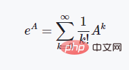
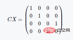
Definition of identity matrix and Pauli matrix

这些是基本的泡利矩阵，这三个两能级体系的泡利矩阵具有非常好的物理性质，如都是酉矩阵且存在特殊的对易关系等：

矩阵指数与旋转门操作

矩阵的指数计算一般采用泰勒级数展开的方法来进行定义：

这里如果我们代入上述介绍的泡利矩阵就会得到这样的结果：

CX门操作的定义

在上述提到的所有的量子门操作中，CX是唯一的一个两比特量子门操作，也就是同时作用在两个量子比特上面，其矩阵形式的定义如下所示：

使用魔法函数__or__来实现量子门操作运算

我们首先简单谈一下为什么要用__or__这个魔法函数而不是其他的二元运算符来实现，这点跟开源库ProjectQ是同步的，理由是我们在量子力学中的运算，一般写成如下的形式：

|ψt〉=U|ψ0〉

将量子态写成狄拉克符号的形式，中文称为"左矢"和"右矢"，英文称之为"bra"和"ket"。因此竖线形式的定义，在形式上会更加契合量子力学的思维，当然，就算是换成其他的符号也是无可厚非的。

功能测试验证

在定义了量子态的类和量子门操作的类之后，我们可以写如下所示的一个测试脚本来测试程序的执行效果：

# TestQubits.py
from QubitPair import QubitPair
from Operator import QubitOperator
 
if __name__ == '__main__':
    qubits = QubitPair()
    print ('The initial state is: {}'.format(qubits))
    QubitOperator('X', 3.1415926, 0) | qubits
    print ('Applying X on the 0th qubit...')
    print ('The new state is: {}'.format(qubits))
    QubitOperator('CX') | qubits
    print ('Applying entanglement on qubits...')
    print ('The new state is: {}'.format(qubits))
    QubitOperator('X', 3.1415926, 0) | qubits
    print ('Applying X on the 0th qubit...')
    print ('The new state is: {}'.format(qubits))
    QubitOperator('CX') | qubits
    print ('Applying entanglement on qubits...')
    print ('The new state is: {}'.format(qubits))

这个程序的测试逻辑为：先定义一个两比特的量子系统，然后对第一个比特执行X门操作，使得其从|0〉态变成|1〉态，再对这两个比特执行纠缠门CX操作，观察其态的变化情况。之后再将第一个比特的状态变回|0〉态，再观察作用CX的态的变化情况，执行结果如下所示：

[dechin@dechin-manjaro simulator]$ python3 TestQubits.py 
The initial state is: [1.+0.j 0.+0.j 0.+0.j 0.+0.j]
Applying X on the 0th qubit...
The new state is: [2.67948966e-08+0.j 0.00000000e+00+0.j 0.00000000e+00-1.j
 0.00000000e+00+0.j]
Applying entanglement on qubits...
The new state is: [2.67948966e-08+0.j 0.00000000e+00+0.j 0.00000000e+00+0.j
 0.00000000e+00-1.j]
Applying X on the 0th qubit...
The new state is: [ 7.17966483e-16+0.00000000e+00j -1.00000000e+00+0.00000000e+00j
  0.00000000e+00-2.67948966e-08j  0.00000000e+00-2.67948966e-08j]
Applying entanglement on qubits...
The new state is: [ 7.17966483e-16+0.00000000e+00j -1.00000000e+00+0.00000000e+00j
  0.00000000e+00-2.67948966e-08j  0.00000000e+00-2.67948966e-08j]

这个结果所展示出来的数字也许比较乱，这是因为在运算过程中的计算精度不足所导致的，这里低于1e-06的数字其实我们可以认为就是0。那么我们从这个结果中可以分析总结出量子态的演变历程：

|00〉⇒|10〉⇒|11〉⇒|01〉⇒|01〉

注意：上面的这种写法，其实不太合乎程序语言的逻辑，一般从右到左的方向才是从低位到高位的写法。因此，严格来说写法应该是：|00〉⇒|01〉⇒|11〉⇒|10〉⇒|10〉。

这里我们就完成了基于魔法函数的量子计算模拟的过程，感兴趣的读者可以自行尝试更多的玩法，这里就不进行更多的测试了！

The above is the detailed content of What are the methods for implementing magic functions and quantum computing simulation in Python?. For more information, please follow other related articles on the PHP Chinese website!