

 Backend DevelopmentPython TutorialCommonly used loss functions and Python implementation examples
What is the loss function?
The loss function is an algorithm that measures the degree of fit between the model and the data. A loss function is a way of measuring the difference between actual measurements and predicted values. The higher the value of the loss function, the more incorrect the prediction is, and the lower the value of the loss function, the closer the prediction is to the true value. The loss function is calculated for each individual observation (data point). The function that averages the values of all loss functions is called the cost function. A simpler understanding is that the loss function is for a single sample, while the cost function is for all samples.
Loss functions and metrics
Some loss functions can also be used as evaluation metrics. But loss functions and metrics have different purposes. While metrics are used to evaluate the final model and compare the performance of different models, the loss function is used during the model building phase as an optimizer for the model being created. The loss function guides the model on how to minimize the error.
That is to say, the loss function knows how the model is trained, and the measurement index explains the performance of the model.
Why use the loss function?
Because the loss function measures is the difference between the predicted value and the actual value, so they can be used to guide model improvement when training the model (the usual gradient descent method). In the process of building the model, if the weight of the feature changes and gets better or worse predictions, it is necessary to use the loss function to judge whether the weight of the feature in the model needs to be changed, and the direction of change.
We can use a variety of loss functions in machine learning, depending on the type of problem we are trying to solve, the data quality and distribution, and the algorithm we use. The following figure shows the 10 we have compiled Common loss functions:

Regression problem
1. Mean square error (MSE)
Mean square error refers to all predicted values and the true values, and average them. Often used in regression problems.
def MSE (y, y_predicted):
 sq_error = (y_predicted - y) ** 2
 sum_sq_error = np.sum(sq_error)
 mse = sum_sq_error/y.size
 return mse
2. Mean absolute error (MAE)
is calculated as the average of the absolute differences between the predicted value and the true value. This is a better measurement than mean squared error when the data has outliers.
def MAE (y, y_predicted):
 error = y_predicted - y
 absolute_error = np.absolute(error)
 total_absolute_error = np.sum(absolute_error)
 mae = total_absolute_error/y.size
 return mae
3. Root mean square error (RMSE)
This loss function is the square root of the mean square error. This is an ideal approach if we don't want to punish larger errors.
def RMSE (y, y_predicted):
 sq_error = (y_predicted - y) ** 2
 total_sq_error = np.sum(sq_error)
 mse = total_sq_error/y.size
 rmse = math.sqrt(mse)
 return rmse
4. Mean deviation error (MBE)
is similar to the mean absolute error but does not seek the absolute value. The disadvantage of this loss function is that negative and positive errors can cancel each other out, so it is better to apply it when the researcher knows that the error only goes in one direction.
def MBE (y, y_predicted):
 error = y_predicted -y
 total_error = np.sum(error)
 mbe = total_error/y.size
 return mbe
5. Huber loss
The Huber loss function combines the advantages of mean absolute error (MAE) and mean square error (MSE). This is because Hubber loss is a function with two branches. One branch is applied to MAEs that match expected values, and the other branch is applied to outliers. The general function of Hubber Loss is:

Here
def hubber_loss (y, y_predicted, delta)
 delta = 1.35 * MAE
 y_size = y.size
 total_error = 0
 for i in range (y_size):
erro = np.absolute(y_predicted[i] - y[i])
if error < delta:
 hubber_error = (error * error) / 2
else:
 hubber_error = (delta * error) / (0.5 * (delta * delta))
total_error += hubber_error
 total_hubber_error = total_error/y.size
 return total_hubber_error
binary classification
6. Maximum Likelihood Loss (Likelihood Loss/LHL)
This loss function is mainly used for binary classification problems. The probability of each predicted value is multiplied to obtain a loss value, and the associated cost function is the average of all observed values. Let us take the following example of binary classification where the class is [0] or [1]. If the output probability is equal to or greater than 0.5, the predicted class is [1], otherwise it is [0]. An example of the output probability is as follows:
[0.3 , 0.7 , 0.8 , 0.5 , 0.6 , 0.4]
The corresponding predicted class is:
[0 , 1 , 1 , 1 , 1 , 0]
and the actual class is:
[0 , 1 , 1 , 0 , 1 , 0]
Now the real class and output probability will be used to calculate loss. If the true class is [1], we use the output probability. If the true class is [0], we use the 1-probability:
((1–0.3)+0.7+0.8+(1–0.5)+0.6+(1–0.4)) / 6 = 0.65
The Python code is as follows:
def LHL (y, y_predicted):
 likelihood_loss = (y * y_predicted) + ((1-y) * (y_predicted))
 total_likelihood_loss = np.sum(likelihood_loss)
 lhl = - total_likelihood_loss / y.size
 return lhl
7. Binary crossover Entropy (BCE)
This function is a modification of the logarithmic likelihood loss. Stacking sequences of numbers can penalize highly confident but incorrect predictions. The general formula for the binary cross-entropy loss function is:

Let’s continue using the values from the above example:
- Output probability = [0.3, 0.7, 0.8, 0.5, 0.6, 0.4]
- Actual class = [0, 1, 1, 0, 1, 0]
- (0 . log (0.3) (1–0) . log (1–0.3)) = 0.155
- (1 . log(0.7) (1–1) . log (0.3)) = 0.155
- (1 . log(0.8) (1–1) . log (0.2)) = 0.097
- (0 . log (0.5) (1–0) . log (1–0.5) ) = 0.301
- (1 . log(0.6) (1–1) . log (0.4)) = 0.222
- (0 . log (0.4) (1–0) . log ( 1–0.4)) = 0.222
Then the result of the cost function is:
(0.155 + 0.155 + 0.097 + 0.301 + 0.222 + 0.222) / 6 = 0.192
The Python code is as follows:
def BCE (y, y_predicted):
 ce_loss = y*(np.log(y_predicted))+(1-y)*(np.log(1-y_predicted))
 total_ce = np.sum(ce_loss)
 bce = - total_ce/y.size
 return bce
8, Hinge Loss and Squared Hinge Loss (HL and SHL)
Hinge Loss is translated as hinge loss or hinge loss. English shall prevail here.
Hinge Loss主要用于支持向量机模型的评估。错误的预测和不太自信的正确预测都会受到惩罚。所以一般损失函数是:

这里的t是真实结果用[1]或[-1]表示。
使用Hinge Loss的类应该是[1]或-1。为了在Hinge loss函数中不被惩罚,一个观测不仅需要正确分类而且到超平面的距离应该大于margin(一个自信的正确预测)。如果我们想进一步惩罚更高的误差,我们可以用与MSE类似的方法平方Hinge损失,也就是Squared Hinge Loss。
如果你对SVM比较熟悉,应该还记得在SVM中,超平面的边缘(margin)越高,则某一预测就越有信心。如果这块不熟悉,则看看这个可视化的例子:

如果一个预测的结果是1.5,并且真正的类是[1],损失将是0(零),因为模型是高度自信的。
loss= Max (0,1 - 1* 1.5) = Max (0, -0.5) = 0

如果一个观测结果为0(0),则表示该观测处于边界(超平面),真实的类为[-1]。损失为1,模型既不正确也不错误,可信度很低。


如果一次观测结果为2,但分类错误(乘以[-1]),则距离为-2。损失是3(非常高),因为我们的模型对错误的决策非常有信心(这个是绝不能容忍的)。

python代码如下:
#Hinge Loss
def Hinge (y, y_predicted):
 hinge_loss = np.sum(max(0 , 1 - (y_predicted * y)))
 return hinge_loss

#Squared Hinge Loss
def SqHinge (y, y_predicted):
 sq_hinge_loss = max (0 , 1 - (y_predicted * y)) ** 2
 total_sq_hinge_loss = np.sum(sq_hinge_loss)
 return total_sq_hinge_loss
多分类
9、交叉熵(CE)
在多分类中,我们使用与二元交叉熵类似的公式,但有一个额外的步骤。首先需要计算每一对[y, y_predicted]的损失,一般公式为:

如果我们有三个类,其中单个[y, y_predicted]对的输出是:

这里实际的类3(也就是值=1的部分),我们的模型对真正的类是3的信任度是0.7。计算这损失如下:

为了得到代价函数的值,我们需要计算所有单个配对的损失,然后将它们相加最后乘以[-1/样本数量]。代价函数由下式给出:

使用上面的例子,如果我们的第二对:

那么成本函数计算如下:

使用Python的代码示例可以更容易理解;
def CCE (y, y_predicted):
 cce_class = y * (np.log(y_predicted))
 sum_totalpair_cce = np.sum(cce_class)
 cce = - sum_totalpair_cce / y.size
 return cce
10、Kullback-Leibler 散度 (KLD)
又被简化称为KL散度,它类似于分类交叉熵,但考虑了观测值发生的概率。如果我们的类不平衡,它特别有用。

def KL (y, y_predicted):
 kl = y * (np.log(y / y_predicted))
 total_kl = np.sum(kl)
 return total_kl
以上就是常见的10个损失函数,希望对你有所帮助。
The above is the detailed content of Commonly used loss functions and Python implementation examples. For more information, please follow other related articles on the PHP Chinese website!

 特斯拉自动驾驶算法和模型解读Apr 11, 2023 pm 12:04 PM
特斯拉是一个典型的AI公司,过去一年训练了75000个神经网络,意味着每8分钟就要出一个新的模型,共有281个模型用到了特斯拉的车上。接下来我们分几个方面来解读特斯拉FSD的算法和模型进展。01 感知 Occupancy Network特斯拉今年在感知方面的一个重点技术是Occupancy Network (占据网络)。研究机器人技术的同学肯定对occupancy grid不会陌生,occupancy表示空间中每个3D体素(voxel)是否被占据,可以是0/1二元表示,也可以是[0, 1]之间的
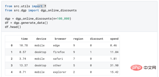 基于因果森林算法的决策定位应用Apr 08, 2023 am 11:21 AM
译者 | 朱先忠审校 | 孙淑娟在我之前的博客中,我们已经了解了如何使用因果树来评估政策的异质处理效应。如果你还没有阅读过,我建议你在阅读本文前先读一遍,因为我们在本文中认为你已经了解了此文中的部分与本文相关的内容。为什么是异质处理效应(HTE:heterogenous treatment effects)呢?首先,对异质处理效应的估计允许我们根据它们的预期结果(疾病、公司收入、客户满意度等)选择提供处理(药物、广告、产品等)的用户(患者、用户、客户等)。换句话说,估计HTE有助于我
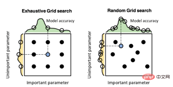 Mango:基于Python环境的贝叶斯优化新方法Apr 08, 2023 pm 12:44 PM
译者 | 朱先忠审校 | 孙淑娟引言模型超参数(或模型设置)的优化可能是训练机器学习算法中最重要的一步,因为它可以找到最小化模型损失函数的最佳参数。这一步对于构建不易过拟合的泛化模型也是必不可少的。优化模型超参数的最著名技术是穷举网格搜索和随机网格搜索。在第一种方法中,搜索空间被定义为跨越每个模型超参数的域的网格。通过在网格的每个点上训练模型来获得最优超参数。尽管网格搜索非常容易实现,但它在计算上变得昂贵,尤其是当要优化的变量数量很大时。另一方面,随机网格搜索是一种更快的优化方法,可以提供更好的
 因果推断主要技术思想与方法总结Apr 12, 2023 am 08:10 AM
导读:因果推断是数据科学的一个重要分支,在互联网和工业界的产品迭代、算法和激励策略的评估中都扮演者重要的角色,结合数据、实验或者统计计量模型来计算新的改变带来的收益,是决策制定的基础。然而,因果推断并不是一件简单的事情。首先,在日常生活中,人们常常把相关和因果混为一谈。相关往往代表着两个变量具有同时增长或者降低的趋势,但是因果意味着我们想要知道对一个变量施加改变的时候会发生什么样的结果,或者说我们期望得到反事实的结果,如果过去做了不一样的动作,未来是否会发生改变?然而难点在于,反事实的数据往往是
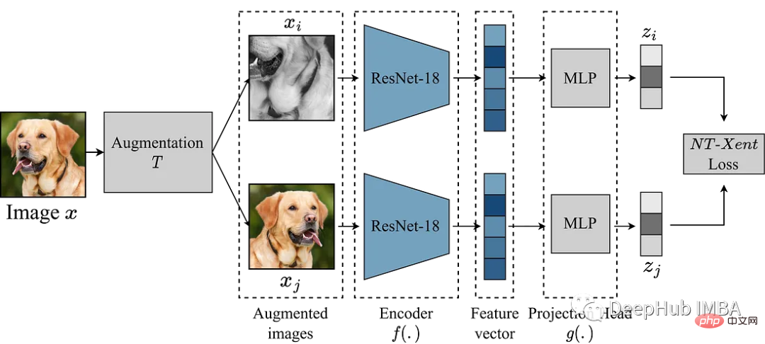 使用Pytorch实现对比学习SimCLR 进行自监督预训练Apr 10, 2023 pm 02:11 PM
SimCLR(Simple Framework for Contrastive Learning of Representations)是一种学习图像表示的自监督技术。 与传统的监督学习方法不同,SimCLR 不依赖标记数据来学习有用的表示。 它利用对比学习框架来学习一组有用的特征,这些特征可以从未标记的图像中捕获高级语义信息。SimCLR 已被证明在各种图像分类基准上优于最先进的无监督学习方法。 并且它学习到的表示可以很容易地转移到下游任务,例如对象检测、语义分割和小样本学习,只需在较小的标记
 盒马供应链算法实战Apr 10, 2023 pm 09:11 PM
一、盒马供应链介绍1、盒马商业模式盒马是一个技术创新的公司,更是一个消费驱动的公司,回归消费者价值:买的到、买的好、买的方便、买的放心、买的开心。盒马包含盒马鲜生、X 会员店、盒马超云、盒马邻里等多种业务模式,其中最核心的商业模式是线上线下一体化,最快 30 分钟到家的 O2O(即盒马鲜生)模式。2、盒马经营品类介绍盒马精选全球品质商品,追求极致新鲜;结合品类特点和消费者购物体验预期,为不同品类选择最为高效的经营模式。盒马生鲜的销售占比达 60%~70%,是最核心的品类,该品类的特点是用户预期时
 研究表明强化学习模型容易受到成员推理攻击Apr 09, 2023 pm 08:01 PM
译者 | 李睿 审校 | 孙淑娟随着机器学习成为人们每天都在使用的很多应用程序的一部分,人们越来越关注如何识别和解决机器学习模型的安全和隐私方面的威胁。 然而,不同机器学习范式面临的安全威胁各不相同,机器学习安全的某些领域仍未得到充分研究。尤其是强化学习算法的安全性近年来并未受到太多关注。 加拿大的麦吉尔大学、机器学习实验室(MILA)和滑铁卢大学的研究人员开展了一项新研究,主要侧重于深度强化学习算法的隐私威胁。研究人员提出了一个框架,用于测试强化学习模型对成员推理攻击的脆弱性。 研究
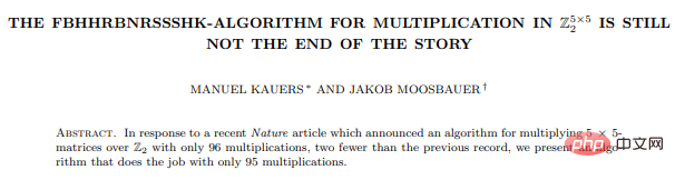 人类反超 AI:DeepMind 用 AI 打破矩阵乘法计算速度 50 年记录一周后,数学家再次刷新Apr 11, 2023 pm 01:16 PM
10 月 5 日,AlphaTensor 横空出世,DeepMind 宣布其解决了数学领域 50 年来一个悬而未决的数学算法问题,即矩阵乘法。AlphaTensor 成为首个用于为矩阵乘法等数学问题发现新颖、高效且可证明正确的算法的 AI 系统。论文《Discovering faster matrix multiplication algorithms with reinforcement learning》也登上了 Nature 封面。然而,AlphaTensor 的记录仅保持了一周,便被人类


Hot AI Tools

Undresser.AI Undress
AI-powered app for creating realistic nude photos

AI Clothes Remover
Online AI tool for removing clothes from photos.

Undress AI Tool
Undress images for free

Clothoff.io
AI clothes remover

AI Hentai Generator
Generate AI Hentai for free.

Hot Article
Hot Tools

EditPlus Chinese cracked version
Small size, syntax highlighting, does not support code prompt function

ZendStudio 13.5.1 Mac
Powerful PHP integrated development environment

Safe Exam Browser
Safe Exam Browser is a secure browser environment for taking online exams securely. This software turns any computer into a secure workstation. It controls access to any utility and prevents students from using unauthorized resources.

Dreamweaver Mac version
Visual web development tools

VSCode Windows 64-bit Download
A free and powerful IDE editor launched by Microsoft

