How to apply Python in cohort analysis

Cohort Analysis

Cohort Analysis Concept

Cohort literally means a group of people (with common characteristics or similar behaviors), such as different genders and different ages.

Cohort analysis: Compares changes in similar groups over time.

The product will continue to iterate as you develop and test it, which results in users who join in the first week of product release having a different experience than those who join later. For example, each user will go through a life cycle: from free trial, to paid use, and finally stop using it. At the same time, during this period, you are constantly making adjustments to your business model. Therefore, users who “eat crabs” in the first month after the product is launched are bound to have a different onboarding experience than users who join after four months. What impact will this have on churn rates? We used cohort analysis to find out.

Each group of users forms a cohort and participates in the entire experimental process. By comparing different cohorts, you can learn whether overall performance on key metrics is getting better.

Combined with the user analysis level, such as users acquired in different months, new users from different channels, and users with different characteristics (such as users on WeChat who communicate with at least 10 friends on WeChat every day).

Cohort Analysis is a comparative analysis of these groups of people with different characteristics to discover their behavioral differences in the time dimension.

Therefore, cohort analysis is mainly used for the following two points:

• Compare the data indicators of different cohort groups in the same experience cycle to verify the effect of product iteration optimization

• Compare the data indicators of different experience cycles (life cycles) of the same cohort group and discover the problem of long-term experience

We are conducting cohort analysis At this time, it can be roughly divided into two processes: determining the grouping logic of the cohort and determining the key data indicators of the cohort analysis.

• Groups with similar behavioral characteristics

• Groups with the same time period

For example:

1. By customer acquisition month (grouped by week or even day)

2. By customer acquisition channel

3. Category according to the specific actions completed by the user, such as the number of times the user visits the website or the number of purchases.

Regarding key data indicators, they need to be based on the time dimension, such as retention, revenue, self-propagation coefficient, etc.

The following is a case example using retention rate as an indicator:

The following is the operating data of an e-commerce company. We will use this data to demonstrate using python Cohort analysis.

Detailed explanation of cohort analysis case:

The data is an e-commerce user's payment log. The log fields include date, payment amount and user ID, which have been desensitized.

Data reading

import pandas as pd

df = pd.read_csv('日志.csv', encoding="gb18030")
df.head()

Analysis direction

Group logic:

Here only based on the user’s initial purchase month For grouping, if the log contains more classification fields (such as channel, gender or age, etc.), you can consider more grouping logic.

Key data indicators:

For this data, there are at least 3 data indicators that can be analyzed:

1. Retention Rate

2. Payment amount per capita

3. Number of purchases per capita

Data preprocessing

Because we are grouping by month, we need to resample the dates into months first:

df['购买月份'] = pd.to_datetime(df.日期).dt.to_period("M")
df.head()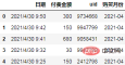

Calculate the total payment of each user in each month:

order = df.groupby(["uid", "购买月份"], as_index=False).agg(
    月付费总额=("付费金额","sum"),
    月付费次数=("uid","count"),
)
order.head()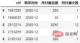

Calculate the first purchase month of each user as a cohort group, and map it to the original data:

order["首单月份"] = order.groupby("uid")['购买月份'].transform("min")
order.head()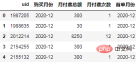

Calculate the month difference between the time of each purchase record and the first purchase time, and reset the month difference label:

order["标签"] = (order.购买月份-order.首单月份).apply(lambda x:"同期群人数" if x.n==0 else f"+{x.n}月")
order.head()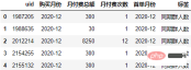

Both months are Period type, after subtraction, a column of object type is obtained, and the type of each element of this column is pandas._libs.tslibs.offsets.MonthEnd

The MonthEnd type has an attribute n that can return a specific difference integer.

Cohort analysis

We said earlier that there are at least 3 data indicators that can be analyzed:

1. Retention rate

2. Payment amount per person

3. Number of purchases per person

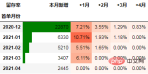
从留存率角度进行同期群分析

通过数据透视表可以一次性计算所需的数据：

cohort_number = order.pivot_table(index="首单月份", columns="标签",
                             values="uid", aggfunc="count",
                             fill_value=0).rename_axis(columns="留存率")
cohort_number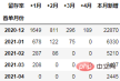

注意：rename_axis(columns=None)用于删除列标签的轴名称。rename_axis(columns=“留存率”)则设置轴名称为留存率。

将 本月新增 列移动到第一列：

cohort_number.insert(0, "同期群人数", cohort_number.pop("同期群人数"))
cohort_number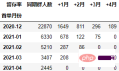

具体过程是先通过pop删除该列，然后插入到0位置，并命名为指定的列名。

 在本次的分析中，留存率的具体计算方式为：+N月留存率=+N月付款用户数/首月付款用户数

cohort_number.iloc[:, 1:] = cohort_number.iloc[:, 1:].divide(cohort_number.本月新增, axis=0)
cohort_number

以百分比形式显示，并设置颜色：

out1 = (cohort_number.style
        .format("{:.2%}", subset=cohort_number.columns[1:])
        .bar(subset="同期群人数", color="green")
        .background_gradient("Reds", subset=cohort_number.columns[1:], high=1, axis=None)
        )
out1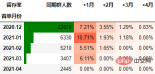

至此计算完毕。

从人均付款金额角度进行同期群分析

要从从人均付款金额角度考虑，需要考虑同期群基期这个整体。具体计算方式是先计算各月的付款总额，然后除以基期的总人数：

cohort_amount = order.pivot_table(index="首单月份", columns="标签",
                                  values="月付费总额", aggfunc="sum",
                                  fill_value=0).rename_axis(columns="人均付款金额")
cohort_amount.insert(0, "首月人均付费", cohort_amount.pop("同期群人数"))
cohort_amount.insert(0, "同期群人数", cohort_number.同期群人数)
cohort_amount.iloc[:, 1:] = cohort_amount.iloc[:, 1:].divide(cohort_amount.同期群人数, axis=0)
out2 = (cohort_amount.style
        .format("{:.2f}", subset=cohort_amount.columns[1:])
        .background_gradient("Reds", subset=cohort_amount.columns[1:], axis=None)
        .bar(subset="同期群人数", color="green")
        )
out2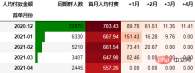

可以看到，12月份的同期群首月新用户人均消费为703.43元，然后逐月递减，到+4月后这些用户人均消费仅11.41元。而随着版本的迭代发展，新增用户的首月消费并没有较大提升，且接下来的消费趋势反而不如12月份。由此可见产品的发展受到了一定的瓶颈，需要思考增长营收的出路了。

一般来说， 通过同期群分析可以比较好指导我们后续更深入细致的数据分析，为产品优化提供参考。

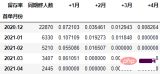
从人均购买次数角度进行同期群分析

依然按照上面一样的套路：

cohort_count = order.pivot_table(index="首单月份", columns="标签",
                                 values="月付费次数", aggfunc="sum",
                                 fill_value=0).rename_axis(columns="人均购买次数")
cohort_count.insert(0, "首月人均频次", cohort_count.pop("同期群人数"))
cohort_count.insert(0, "同期群人数", cohort_number.同期群人数)
cohort_count.iloc[:, 1:] = cohort_count.iloc[:,
                                             1:].divide(cohort_count.同期群人数, axis=0)
out3 = (cohort_count.style
        .format("{:.2f}", subset=cohort_count.columns[1:])
        .background_gradient("Reds", subset=cohort_count.columns[1:], axis=None)
        .bar(subset="同期群人数", color="green")
        )
out3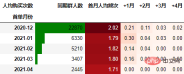

可以得到类似上述一致的结论。

每月总体付费情况

下面我们看看每个月的总体消费情况：

order.groupby("购买月份").agg(
    付费人数=("uid", "count"),
    人均付款金额=("月付费总额", "mean"),
    月付费总额=("月付费总额", "sum")
)

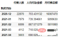
可以看到总体付费人数和付费金额都在逐月下降。

将结果导出网页或截图

对于Styler类型，我们可以调用render方法转化为网页源代码，通过以下方式即可将其导入到一个网页文件中：

with open("out.html", "w") as f:
    f.write(out1.render())
    f.write(out2.render())
    f.write(out3.render())

如果你的电脑安装了谷歌游览器，还可以安装dataframe_image，将这个表格导出为图片。

安装：pip install dataframe_image

import dataframe_image as dfi

dfi.export(obj=out1, filename='留存率.jpg')
dfi.export(obj=out2, filename='人均付款金额.jpg')
dfi.export(obj=out3, filename='人均购买次数.jpg')

dfi.export的参数：

• obj : 被导出的Datafream对象

• filename : 文件保存位置

• fontsize : 字体大小

• max_rows : 最大行数

• max_cols : 最大列数

• table_conversion : 使用谷歌游览器或原生’matplotlib’, 只要写非’chrome’的值就会使用原生’matplotlib’

• chrome_path : 指定谷歌游览器位置

 整体完整代码

import pandas as pd
import dataframe_image as dfi

df = pd.read_csv('日志.csv', encoding="gb18030")
df['购买月份'] = pd.to_datetime(df.日期).dt.to_period("M")
order = df.groupby(["uid", "购买月份"], as_index=False).agg(
    月付费总额=("付费金额", "sum"),
    月付费次数=("uid", "count"),
)
order["首单月份"] = order.groupby("uid")['购买月份'].transform("min")
order["标签"] = (
    order.购买月份-order.首单月份).apply(lambda x: "同期群人数" if x.n == 0 else f"+{x.n}月")
cohort_number = order.pivot_table(index="首单月份", columns="标签",
                                  values="uid", aggfunc="count",
                                  fill_value=0).rename_axis(columns="留存率")
cohort_number.insert(0, "同期群人数", cohort_number.pop("同期群人数"))
cohort_number.iloc[:, 1:] = cohort_number.iloc[:,1:].divide(cohort_number.同期群人数, axis=0)
out1 = (cohort_number.style
        .format("{:.2%}", subset=cohort_number.columns[1:])
        .bar(subset="同期群人数", color="green")
        .background_gradient("Reds", subset=cohort_number.columns[1:], high=1, axis=None)
        )
cohort_amount = order.pivot_table(index="首单月份", columns="标签",
                                  values="月付费总额", aggfunc="sum",
                                  fill_value=0).rename_axis(columns="人均付款金额")
cohort_amount.insert(0, "首月人均付费", cohort_amount.pop("同期群人数"))
cohort_amount.insert(0, "同期群人数", cohort_number.同期群人数)
cohort_amount.iloc[:, 1:] = cohort_amount.iloc[:, 1:].divide(cohort_amount.同期群人数, axis=0)
out2 = (cohort_amount.style
        .format("{:.2f}", subset=cohort_amount.columns[1:])
        .background_gradient("Reds", subset=cohort_amount.columns[1:], axis=None)
        .bar(subset="同期群人数", color="green")
        )
cohort_count = order.pivot_table(index="首单月份", columns="标签",
                                 values="月付费次数", aggfunc="sum",
                                 fill_value=0).rename_axis(columns="人均购买次数")
cohort_count.insert(0, "首月人均频次", cohort_count.pop("同期群人数"))
cohort_count.insert(0, "同期群人数", cohort_number.同期群人数)
cohort_count.iloc[:, 1:] = cohort_count.iloc[:,
                                             1:].divide(cohort_count.同期群人数, axis=0)
out3 = (cohort_count.style
        .format("{:.2f}", subset=cohort_count.columns[1:])
        .background_gradient("Reds", subset=cohort_count.columns[1:], axis=None)
        .bar(subset="同期群人数", color="green")
        )
outs = [out1, out2, out3]
with open("out.html", "w") as f:
    for out in outs:
        f.write(out.render())
        display(out)

dfi.export(obj=out1, filename='留存率.jpg')
dfi.export(obj=out2, filename='人均付款金额.jpg')
dfi.export(obj=out3, filename='人均购买次数.jpg')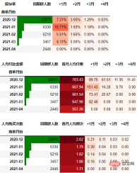

The above is the detailed content of How to apply Python in cohort analysis. For more information, please follow other related articles on the PHP Chinese website!