Digital twin modeling based on machine learning and constrained optimization

Translator | Zhu Xianzhong

Reviewer | Sun Shujuan

Introduction

Today, data science is widely used to create digital twins (Digital Twins) - digital twins It is the digital counterpart of a real-world physical system or process and can be used for simulation and prediction of input behavior, monitoring, maintenance, planning, etc. While digital twins such as cognitive customer service bots are common in everyday applications, in this article I will compare the two different types for modeling by illustrating two different types of digital twins in industry Twin data science technology.

Two widely used data science areas of digital twins discussed in this article are as follows:

a) Diagnostic and Predictive Analysis: In this analysis method, given A series of inputs used by the digital twin to diagnose the cause or predict the future behavior of the system. IoT-based machine learning models are used to create smart machines and factories. This model allows sensor inputs to be analyzed in real time to diagnose, predict and prevent future problems and failures before they occur.

b) Prescriptive Analysis: This analysis method simulates the entire network so that, given a set of variables and constraints to be adhered to, from Determine the best or feasible solution among a large number of candidates, usually with the goal of maximizing stated business goals such as throughput, utilization, output, etc. These optimization problems are widely used in the field of supply chain planning and scheduling, such as when a logistics provider creates a schedule for its resources (vehicles, personnel) in order to maximize on-time delivery; also when a manufacturer creates a schedule so that Optimize the use of machines and operators to achieve maximum OTIF (On Time In Full) delivery. The data science technique used here is constrained mathematical optimization, an algorithm that uses powerful solvers to solve complex decision-driven problems.

In summary, ML models predict possible outcomes for a given set of input features based on historical data, and optimization models help you decide, if the predicted outcome occurs, how you should plan to solve/mitigate/exploit it, because Your business has several potentially competing goals that you may choose to pursue with limited resources.

These two fields of data science, while sharing some tools (such as Python libraries), mobilize data scientists with completely different skill sets - they often require different ways of thinking and modeling business problems. So, let’s try to understand and compare the methods involved so that a data scientist experienced in one domain can understand and cross-utilize skills and techniques that may be applicable in another domain.

Digital Twin Model Application Case

For comparison, let us consider a twin model of a ML-based production root cause analysis (RCA: Root Cause Analysis) process, the purpose of which is to diagnose the finished product or The root cause of defects or anomalies discovered during manufacturing. This will help department managers eliminate the most likely root causes based on the tool’s predictions, ultimately identify issues and implement CAPA (Corrective & Preventive actions: corrective and preventive actions), and browse all machine maintenance records quickly and without spending much manpower. , operator history records, process SOP (Standard Operating Procedure: Standard Operating Procedure), IoT sensor input, etc. The goal is to minimize machine downtime, production losses and improve resource utilization.

Technically, this can be considered a multi-category classification problem. In this problem, assuming a certain defect exists, the model attempts to predict the probability of each of a set of possible root cause labels, such as machine-related, operator-related, process-instruction-related, raw-material-related, or something else. , as well as fine-grained reasons such as machine calibration, machine maintenance, operator skills, operator training, etc. under these first-level classification labels. Although the optimal solution to this situation requires the evaluation of several complex ML models, to emphasize the purpose of this article, let's simplify a bit - assume this is a multinomial logistic regression problem (for reasons that will become clear in the next section).

For comparison, let us consider an optimized twin model of the production planning process, which generates a schedule based on machines, operators, process steps, durations, raw material arrival schedules, due dates, etc. , attempts to maximize an objective such as output or revenue. Such automated timelines help organizations quickly adjust resources to respond to new opportunities from the market (such as demand for drugs due to COVID-19) or to maximize the impact of their raw materials, suppliers, logistics providers, and customer/market mix. Minimize the impact of unforeseen events, such as recent supply chain bottlenecks.

At a basic level for modeling any business problem, developing such a digital twin requires consideration of the following factors:

A. Input features or dimensions

B. Input data— —The values ​​of these dimensions

C, input to output transformation rules

D, output or target

Next, let’s analyze and compare machine learning in more depth ( ML) and optimize these factors in the model under constraints:

A. Input features: These are data dimensions in the system, suitable for both ML and optimization. For an ML model trying to diagnose problems in a production process, features to consider might include: IoT inputs, historical machine maintenance data, operator skills and training information, raw material quality information, SOPs followed (Standard Operating Procedures) Procedure) and other contents.

Similarly, in an optimization environment under constraints, characteristics that need to be considered would include: equipment availability, operator availability, raw material availability, working hours, productivity, skills, etc. that are typically required to develop an optimal production plan feature.

B. Input data: This is where the above two methods use eigenvalues ​​in significantly different ways. Among them, ML models require a large amount of historical data for training. However, significant work related to data preparation, management, and normalization is often required before data can be fed into a model. It is important to note that a history is a record of an event that actually occurred (such as a machine failure or an operator skill issue that resulted in insufficient output), but is usually not a simple combination of all possible values ​​that these characteristics can obtain. In other words, the transaction history will contain more records for those scenarios that occur frequently, while relatively few records for some other scenarios—perhaps less for scenarios that rarely occur. The goal of training a model is to learn the relationship between features and output labels and to predict accurate labels—even when there are few or no feature values ​​or combinations of feature values ​​in the training data.

On the other hand, for optimization methods, characteristic values ​​are usually kept to their actual data, for example, days, batches, deadlines, raw material availability by date, maintenance schedules, machine changeover times , process steps, operator skills, etc. The key difference from ML models is that input data processing requires generating an index table for every possible valid combination of master data feature values ​​(e.g., days, skills, machines, operators, process types, etc.) to form a list of feasible solutions part. For example, operator A uses machine M1 on the first day of the week, performing step 1 of the process at the skill level of S1, or operator B uses machine M1 on the second day, performing step 1 at the skill level of S2; even for Every possible combination of operator, machine, skill level, date, etc., regardless of whether those combinations actually occurred in the past. This results in a very large set of input data records provided to the optimization engine. The goal of an optimization model is to select a specific combination of eigenvalues ​​that meets the given constraints while maximizing (or minimizing) the objective equation.

C. Input to output conversion rules: This is also a significant difference between the two methods. Although both ML and optimization models are based on advanced mathematical theories, mathematical modeling and programming of complex business problems in optimization methods usually require more effort compared with ML, which will be reflected in the following introduction.

The reason is that in ML, with the help of open source libraries like scikit-learn, frameworks such as Pytorch or Tensorflow, and even ML/deep learning models of cloud service providers, the rules for converting input into output are completely interchangeable. It is up to the model to find, which also includes the task of correcting the loss in order to derive the optimal rules (weights, biases, activation functions, etc.). The primary responsibility of a data scientist is to ensure the quality and completeness of input features and their values.

This is not the case for optimization methods, as the rules for how the inputs interact and are converted into outputs must be written by using detailed equations and then fed to solvers such as Gurobi, CPLEX, etc. in order to find the optimal or possible solutions. Furthermore, formulating business problems as mathematical equations requires a deep understanding of the interrelationships in the modeling process and requires data scientists to work closely with business analysts.

Below, let us illustrate this with a schematic diagram of a logistic regression model for a problem RCA (Root Cause Analysis) application:

Logistic Regression ML Model

Note that in this case, the task of calculating the rules (Zᵢ) to generate results based on the input data is left to the model to deduce, while data scientists are usually busy using well-defined confusion matrices, RMSE and other measurement techniques to Visual approach to achieve accurate predictions.

We can compare this with the way production plans are generated through optimization methods:

(I) The first step is to define the business rules (constraints) that encapsulate the planning process.

The following is an example of a production plan:

First, we define some input variables (some of which can be decision variables, used to drive goals):

• Bᵦ,_p,ᵢ——Binary variable, indicating whether the batch β (in the batch table) of product p (in the product table) is scheduled on the i-th day.
• Oₒ,_p,ᵢ - Binary variable indicating whether the operator at index o (in the operator table) is scheduled to process a batch of product p on day i.
• M_m,_p,ᵢ——Binary variable indicating whether the machine with index m (in the machine table) is scheduled to process a batch on the i-th day Product p.

and some coefficients:

• TOₒ,_p - the time it takes operator o to process a batch of product p.
• TM_m,_p——The time it takes for machine m to process a batch of product p.
• OAvₒ,ᵢ——The number of hours available for operator index o on day i.
• MAv_m,ᵢ——The number of hours available for the machine with index m on day i.

In this case, some constraints (rules) can be implemented using the following:

a) In the plan, a specific batch can only be started once.

Where, for each batch of products, Bt is the total number of batches, Pr is the total number of products, and D is the number of days in the plan:

b) One product Can only be started once per day on an operator or machine.

For each day for each product, where Op is the set of all operators and Mc is the set of all machines:

c) The total time spent on a batch (all products) should not exceed the number of operator and machine hours available for the day.

For each operator, there are the following constraints:

For each day of each machine, there are the following constraints:

d) If an operator processes a batch of product within the first 5 days of the schedule, all other batches of the same product must be assigned to the same operator. This maintains operator continuity and productivity.

For each operator and each product, the following constraints exist for each day d (from the 6th day onwards):

The above are required in the program A few of the hundreds of constraints written to form the business rules for real production scheduling scenarios into mathematical equations. Note that these constraints are linear equations (or, more specifically, mixed integer equations). However, the complexity difference between them and logistic regression ML models is still very obvious.

(II) Once the constraints are determined, the output target needs to be defined. This is a critical step and can be a complex process, as explained in the next section.

(III) Finally, the input decision variables, constraints and objectives are sent to the solver to obtain the solution (schedule).

The schematic diagram describing the digital twin based on the optimization method is as follows:

Optimization model

D, output or Goal: For ML models, depending on the type of problem (classification, regression, clustering), it is possible to well establish outputs and metrics for measuring their accuracy. While I will not delve into these issues in this article, given the wealth of information available, it is worth noting that the output of various models can be evaluated with a high degree of automation, such as that of leading CSPs (AWS Sagemaker, Azure ML, etc.) .

Evaluating whether an optimized model generates the correct output is more challenging. Optimization models work by trying to maximize or minimize a computational expression called an "objective." Like constraints, the goal section is designed by the data scientist based on what the business is trying to achieve. More specifically, this is achieved by attaching reward conditions and penalty conditions to decision variables, the sum of which the optimizer attempts to maximize. For real-world problems, it takes many iterations to find the right weights for different goals in order to find a good balance between sometimes conflicting goals.

To further illustrate the above production scheduling example, we might as well design the following two such goals:

a) The schedule should be loaded in advance; the batches should be scheduled as soon as possible, and the remaining capacity in the plan should be at the end of the plan. We can do this by attaching a one-day penalty to a batch, which will gradually increase each day in the schedule.

b) On the other hand, we also want to group batches of the same product so that the resources (operators and machines) are partially utilized optimally, provided that the batches meet the delivery deadline and the groups are in one run Do not exceed machine capacity. Therefore, we define a Batch_group_bonus that provides a higher bonus (hence the exponential in the expression below) if the batches are arranged in larger groups rather than in smaller groups. It is important to note that this may sometimes intersect with previous targets, as some batches that may start today will be started with more batches that become available in a few days, potentially leaving some unfulfilled early in the schedule. resources utilized.

#Depending on how the solver works, the actual implementation often requires a batch group decision variable. However, this expresses the following concept:

The solver will maximize the objective, that is:

Objective=Batch_group_bonus Day_penalty

Of the above two components of the objective, Which one has a greater impact on a given day of the schedule depends on the weights W₁, W₂ and the dates of the schedule, since the day penalty value will gradually become larger in the later stages of the schedule (higher i values). If the days penalty value is greater than the Batch_group_bonus at some point, the planning solver will find it prudent not to schedule the batch; therefore, even if there is resource capacity in the plan, a zero penalty will be incurred, thus scheduling and incurring a net negative penalty, thereby maximizing the goal. These issues need to be troubleshooted and resolved by data scientists.

Comparison of the relative workload between ML methods and optimization methods

Based on the above discussion, it can be inferred that, generally speaking, optimization projects require more effort than ML projects. Optimization requires extensive data science work at almost every stage of the development process. The specific summary is as follows:

a) Input data processing: In ML and optimization, this is done by data scientists. ML data processing requires selection of relevant features, standardization, discretization, etc. For unstructured data such as text, it can include NLP-based methods such as feature extraction, tokenization, etc. Currently, there are libraries based on multiple languages ​​that can be used for statistical analysis of features as well as dimensionality reduction methods such as PCA.

In optimization, every business and plan has nuances that need to be incorporated into the model. Optimization problems do not deal with historical data, but rather combine every possible data change and identified feature into an index on which decision variables and constraints must depend. Although unlike ML, data processing requires a lot of development work.

b) Model development: As mentioned above, model formulation of optimization solutions requires a lot of effort from data scientists and business analysts to formulate constraints and goals. A solver runs mathematical algorithms, and although it is tasked with solving hundreds or even thousands of equations simultaneously to find a solution, it has no business background.

In ML, model training is highly automated, and algorithms are packaged as open source library APIs or packaged by cloud service providers. Highly complex, pre-trained neural network models based on business-specific data simplify the training task down to the last few layers. Tools like AWS Sagemaker Autopilot or Azure AutoML can even automate the entire process of input data processing, feature selection, training and evaluation of different models and output generation.

c) Testing and Output Processing: In ML, the output of a model can be leveraged with minimal processing. It is generally easy to understand (e.g., the probabilities of different labels), although some effort may be required to introduce other aspects, such as the interpretability of the results. Output and error visualization may also require some effort, but it's not much compared to input processing.

Here too, the optimization problem requires iterative manual testing and validation with the trained eye of a planning expert to assess progress. While the solver attempts to maximize the objective, this in itself often makes little sense from a schedule quality perspective. Unlike ML, one cannot say that a target value above or below a threshold contains a correct or incorrect plan. When a schedule is found to be inconsistent with business objectives, the problem may be related to constraints, decision variables, or objective functions and requires careful analysis to find the cause of anomalies in large and complex schedules.

Additionally, something to consider is the development required to interpret the output of the solver into a human-readable format. The solver takes input decision variables, which are index values ​​of the actual physical entities in the plan, such as batch group index, batch priority index, operator and machine index, and returns the selected values. Reverse processing is required to convert these index values ​​from their respective data frames into a coherent timeline that can be visually presented and analyzed by experts.

d) Finally, even in the operational phase, ML models require much less computation and time to generate observational predictions compared to the training phase. However, the schedule is built from scratch each time and requires the same resources for each run.

The following figure is a rough illustration of the relative workload at each stage of the ML and optimization project:

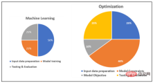
Schematic diagram comparing the relative workload of ML and optimization

Can ML and optimization work together?

Machine learning and optimization solve complementary problems for enterprises; therefore, the output of ML models and optimization reinforce each other and vice versa. AI/ML applications such as IoT predictive maintenance and fault detection, AR/VR remote maintenance and the aforementioned production process RCA form part of the manufacturer’s connected factory strategy.

Optimization applications form the basis of supply chain planning and can be thought of as linking business strategy to operations. They help organizations respond to and plan for unforeseen events. For example, if a problem is detected in a production line, RCA (Root Cause Analysis) tools will help the production line manager quickly narrow down the possible causes and take necessary actions. However, this may sometimes lead to unexpected machine shutdowns or the reassignment of operating instructions. Therefore, production plans may need to be regenerated using available reduced capacity.

Some techniques of ML can be applied to optimization, and vice versa?

Experience from ML projects can be applied to optimization projects; vice versa. For example, for an objective function that is critical to optimizing the output, sometimes the business unit is not as well defined in terms of mathematical modeling as the constraints, which are rules that must be followed and therefore are usually well known. For example, the business objectives are as follows:

a) Batches should be prioritized as early as possible while adhering to delivery deadlines.

b) The schedule should be loaded in advance; the time interval should be scheduled as small as possible and with low resource utilization.

c) Batches should be grouped to efficiently utilize capacity.

d) Operators with higher skill levels for high value products are best assigned such batches.

Some of these goals may have competing priorities that need to be properly balanced, which leads data scientists, when writing complex combinations of influencing factors (such as bonuses and fines), to often focus on what seems to apply to the most common The planning scenarios are accomplished by trial and error; but sometimes the logic is difficult to understand and maintain when flaws arise. Because optimization solvers often use third-party products, their code is often unavailable to the data scientists building the models they want to debug. This makes it impossible to see what values ​​certain bonuses and penalties took on at any particular point in the schedule generation process, and it is these values ​​that make it behave correctly, which makes writing convincing target expressions very important.

Therefore, the above approach helps to adopt the standardization of bonuses and fines, which is a widely used ML practice. The normalized values ​​can then be scaled in a controlled manner using configuration parameters or other means to control the impact of each factor, their relationship to each other, and the values ​​of the preceding and following factors within each of them.

Conclusion

In summary, machine learning and constrained optimization are both advanced mathematical methods for solving different problems in organizations and daily life. They can all be used to deploy digital twins of physical equipment, processes, or network resources. While both types of applications follow similar high-level development processes, ML projects can leverage a high degree of automation available in libraries and cloud-native algorithms, while optimization requires close collaboration between business and data scientists to fully implement the complex planning process. of modeling. Generally speaking, optimization projects require more development work and are resource intensive. In actual development, ML and optimization tools often need to work together in enterprises, and both technologies are useful for data scientists.

Translator Introduction

Zhu Xianzhong, 51CTO community editor, 51CTO expert blogger, lecturer, computer teacher at a university in Weifang, and a veteran in the freelance programming industry.

Original title: ​​Digital Twin Modeling Using Machine Learning and Constrained Optimization​​, author: Partha Sarkar

The above is the detailed content of Digital twin modeling based on machine learning and constrained optimization. For more information, please follow other related articles on the PHP Chinese website!